Introducción a pandas

Pandas es un paquete de Python que proporciona estructuras de datos similares a los dataframes de R. Pandas depende de Numpy, la librería que añade un potente tipo matricial a Python. Los principales tipos de datos que pueden representarse con pandas son:

Datos tabulares con columnas de tipo heterogéneo con etiquetas en columnas y filas.

Series temporales.

Pandas proporciona herramientas que permiten:

Leer y escribir datos en diferentes formatos: CSV, Microsoft Excel, bases SQL y formato HDF5

Seleccionar y filtrar de manera sencilla tablas de datos en función de posición, valor o etiquetas

Fusionar y unir datos

Transformar datos aplicando funciones tanto en global como por ventanas

Manipulación de series temporales

Hacer gráficas

En pandas existen tres tipos básicos de objetos todos ellos basados a su vez en Numpy:

Series (listas, 1D), DataFrame (tablas, 2D) y Panels (tablas 3D).

Revisar otros tutoriales:

https://pandas.pydata.org/pandas-docs/stable/tutorials.html

https://bioinf.comav.upv.es/courses/linux/python/pandas.html

Importar librerias

import pandas as pd
import numpy as np
import matplotlib.pyplot as plt
%matplotlib inline

Lectura del dataset

from google.colab import drive
drive.mount('/content/drive')

Mounted at /content/drive

# Lectura de un dataset (CSV), y almancenamiento en la variable "d"
d = pd.read_csv("/content/drive/MyDrive/Clases 2023-01/Programación Concurrente y Distribuida/Semana 2-3/Introducción a Python/Data/sampledata.csv")

Comandos y operaciones principales de Pandas

# Visualización de los primeros y últimos 5 elementos
d

	id	first_name	last_name	email	country	ip_address	longitude	latitude	age	score
0	1	Sandra	Sims	ssims0@microsoft.com	Armenia	63.84.115.63	44.43054	40.14493	44	0.62
1	2	Anna	Bishop	abishop1@mtv.com	China	204.108.246.11	118.29169	29.67594	90	0.22
2	3	Virginia	Rodriguez	vrodriguez2@so-net.ne.jp	Portugal	88.65.157.43	-8.63330	41.40000	39	0.33
3	4	Julia	Stanley	jstanley3@abc.net.au	China	76.197.170.103	102.19379	38.50062	NaN	0.64
4	5	Jacqueline	Gutierrez	jgutierrez4@shinystat.com	Poland	159.13.71.38	18.54003	54.17062	14	0.50
...	...	...	...	...	...	...	...	...	...	...
995	996	Jean	Payne	jpaynern@bluehost.com	Mexico	191.211.230.212	-92.89380	16.21790	40	0.30
996	997	Michelle	Murphy	mmurphyro@senate.gov	Croatia	129.124.79.138	15.85000	45.78333	87	0.54
997	998	Joseph	Hill	jhillrp@princeton.edu	Japan	161.176.64.135	139.80000	36.41667	50	0.57
998	999	Roger	Harrison	rharrisonrq@gizmodo.com	Poland	7.194.73.231	20.37415	49.84485	18	0.37
999	1000	Kelly	Henry	khenryrr@squidoo.com	Indonesia	145.118.102.45	111.45570	-7.21950	83	0.39

1000 rows × 10 columns

# Ver el tipo de variable de los dataframes de Pandas
type(d)

pandas.core.frame.DataFrame

# Con iloc se puede extraer sólo partes particulares deseadas del dataframe
d.iloc[1:10,3:4]

	email
1	abishop1@mtv.com
2	vrodriguez2@so-net.ne.jp
3	jstanley3@abc.net.au
4	jgutierrez4@shinystat.com
5	nlittle5@latimes.com
6	tfox6@squarespace.com
7	jparker7@gnu.org
8	kwalker8@nba.com
9	wbrown9@boston.com

# Mostrar estadísticas básicas para las variables numéricas
d.describe()

	id	longitude	latitude	score
count	1000.000000	999.000000	999.000000	1000.000000
mean	500.500000	46.831119	24.273880	0.501290
std	288.819436	70.556083	24.272596	0.103403
min	1.000000	-149.333330	-53.787690	0.180000
25%	250.750000	7.046050	8.135695	0.430000
50%	500.500000	42.174440	29.819050	0.510000
75%	750.250000	112.349640	43.186925	0.570000
max	1000.000000	175.496340	72.786840	0.830000

# Acceder a un sólo elemento del dataframe
d.iloc[2,2]

'Rodriguez'

# Acceder a registros seleccionados con todas las columnas
d.iloc[[1,3,5],]

	id	first_name	last_name	email	country	ip_address	longitude	latitude	age	score
1	2	Anna	Bishop	abishop1@mtv.com	China	204.108.246.11	118.29169	29.67594	90	0.22
3	4	Julia	Stanley	jstanley3@abc.net.au	China	76.197.170.103	102.19379	38.50062	NaN	0.64
5	6	Nicole	Little	nlittle5@latimes.com	Panama	235.246.1.116	-78.13774	8.40693	10	0.30

# Seleccionar los primeros diez registros, luego seleccionar solamente 3 columnas
d.iloc[range(10),][["last_name", "country", "score"]]

	last_name	country	score
0	Sims	Armenia	0.62
1	Bishop	China	0.22
2	Rodriguez	Portugal	0.33
3	Stanley	China	0.64
4	Gutierrez	Poland	0.50
5	Little	Panama	0.30
6	Fox	Iran	0.33
7	Parker	China	0.55
8	Walker	Slovenia	0.50
9	Brown	Ethiopia	0.41

# Filtrar el dataset para sólo obtener edades iguales a 44 años
d[d.age=='44']

	id	first_name	last_name	email	country	ip_address	longitude	latitude	age	score
0	1	Sandra	Sims	ssims0@microsoft.com	Armenia	63.84.115.63	44.43054	40.14493	44	0.62
169	170	Jason	Stevens	jstevens4p@foxnews.com	Czech Republic	105.101.112.178	16.11480	50.26742	44	0.54
188	189	Ruby	Gonzales	rgonzales58@pbs.org	Portugal	122.247.105.164	-8.91670	38.70000	44	0.58
251	252	Deborah	Patterson	dpatterson6z@salon.com	Palau	177.16.160.109	134.71725	8.08228	44	0.61
337	338	Todd	Henderson	thenderson9d@latimes.com	Indonesia	4.45.250.25	113.48740	-8.28670	44	0.53
473	474	Nicholas	Scott	nscottd5@samsung.com	Russia	165.111.40.207	104.24940	56.70320	44	0.37
550	551	Kathy	Burke	kburkefa@pen.io	Indonesia	197.17.149.125	115.11730	-8.46090	44	0.73
706	707	Kathryn	Mitchell	kmitchelljm@boston.com	Azerbaijan	113.1.57.57	50.04002	40.56441	44	0.66
723	724	Aaron	Chapman	achapmank3@mayoclinic.com	Indonesia	59.111.140.158	106.02910	-6.74290	44	0.39
843	844	Diana	Bennett	dbennettnf@wikipedia.org	Cuba	147.157.224.46	-74.15181	20.24673	44	0.46

# Ver el tipo de datos almacenados en una columna: dtype('O') para Objetos o Strings
d['age'].dtype

dtype('O')

# Filtrar el dataset para obtener los registros cuando las edades son de 55 o 44 años
d[np.logical_or(d.age=="55", d.age=="44")]

	id	first_name	last_name	email	country	ip_address	longitude	latitude	age	score
0	1	Sandra	Sims	ssims0@microsoft.com	Armenia	63.84.115.63	44.43054	40.14493	44	0.62
18	19	Jimmy	Robertson	jrobertsoni@thetimes.co.uk	Tajikistan	184.90.118.60	68.44668	37.56702	55	0.60
72	73	Michael	Powell	mpowell20@youtube.com	China	232.233.196.224	120.21400	27.32734	55	0.59
169	170	Jason	Stevens	jstevens4p@foxnews.com	Czech Republic	105.101.112.178	16.11480	50.26742	44	0.54
188	189	Ruby	Gonzales	rgonzales58@pbs.org	Portugal	122.247.105.164	-8.91670	38.70000	44	0.58
251	252	Deborah	Patterson	dpatterson6z@salon.com	Palau	177.16.160.109	134.71725	8.08228	44	0.61
266	267	Gerald	Butler	gbutler7e@google.fr	Philippines	149.199.214.71	121.41470	14.12840	55	0.55
337	338	Todd	Henderson	thenderson9d@latimes.com	Indonesia	4.45.250.25	113.48740	-8.28670	44	0.53
367	368	Philip	Harvey	pharveya7@wsj.com	Portugal	188.30.85.41	-8.16630	37.86690	55	0.18
381	382	Joan	Oliver	joliveral@chicagotribune.com	Russia	98.144.120.116	38.40172	54.03481	55	0.37
418	419	Paula	Fowler	pfowlerbm@apache.org	Philippines	221.234.139.145	120.65190	17.56470	55	0.43
473	474	Nicholas	Scott	nscottd5@samsung.com	Russia	165.111.40.207	104.24940	56.70320	44	0.37
550	551	Kathy	Burke	kburkefa@pen.io	Indonesia	197.17.149.125	115.11730	-8.46090	44	0.73
685	686	Jesse	Freeman	jfreemanj1@wikia.com	Iran	66.31.71.144	60.21430	26.22580	55	0.32
706	707	Kathryn	Mitchell	kmitchelljm@boston.com	Azerbaijan	113.1.57.57	50.04002	40.56441	44	0.66
723	724	Aaron	Chapman	achapmank3@mayoclinic.com	Indonesia	59.111.140.158	106.02910	-6.74290	44	0.39
843	844	Diana	Bennett	dbennettnf@wikipedia.org	Cuba	147.157.224.46	-74.15181	20.24673	44	0.46
853	854	Willie	Ross	wrossnp@networkadvertising.org	Indonesia	90.176.105.5	125.18950	1.45697	55	0.53
897	898	Julie	Mason	jmasonox@wikia.com	Libya	229.225.235.75	12.72778	32.75222	55	0.46

# Seleccionar un conjunto de registros del 0 al 9
d.iloc[range(10),]

	id	first_name	last_name	email	country	ip_address	longitude	latitude	age	score
0	1	Sandra	Sims	ssims0@microsoft.com	Armenia	63.84.115.63	44.43054	40.14493	44	0.62
1	2	Anna	Bishop	abishop1@mtv.com	China	204.108.246.11	118.29169	29.67594	90	0.22
2	3	Virginia	Rodriguez	vrodriguez2@so-net.ne.jp	Portugal	88.65.157.43	-8.63330	41.40000	39	0.33
3	4	Julia	Stanley	jstanley3@abc.net.au	China	76.197.170.103	102.19379	38.50062	NaN	0.64
4	5	Jacqueline	Gutierrez	jgutierrez4@shinystat.com	Poland	159.13.71.38	18.54003	54.17062	14	0.50
5	6	Nicole	Little	nlittle5@latimes.com	Panama	235.246.1.116	-78.13774	8.40693	10	0.30
6	7	Terry	Fox	tfox6@squarespace.com	Iran	81.219.197.208	55.49164	37.38071	89	0.33
7	8	Jeremy	Parker	jparker7@gnu.org	China	17.207.110.163	110.71266	22.01041	60	0.55
8	9	Kenneth	Walker	kwalker8@nba.com	Slovenia	117.248.31.17	13.97028	45.68472	no disponible	0.50
9	10	Willie	Brown	wbrown9@boston.com	Ethiopia	253.51.12.171	42.80000	9.35000	17	0.41

# Verificar que el tipo de variable sigue siendo dataframe
type(d.iloc[range(10),])

pandas.core.frame.DataFrame

# Obtener sólo una columna como una Serie
d.age

0       44
1       90
2       39
3      NaN
4       14
      ... 
995     40
996     87
997     50
998     18
999     83
Name: age, Length: 1000, dtype: object

# Ver tipo de dato, ahora ya no es dataframe, sinó una serie
type(d.age)

pandas.core.series.Series

d["score"].dtype, d['age'].dtype

(dtype('float64'), dtype('O'))

# Crear una nueva columna llamada "scoretimes2", que será la columna score multiplicada por 2
d["scoretimes2"] = d["score"]*2

# Visualizar los primeros 10 elementos, ahora con la nueva columna al final (scoretimes2)
d.head(10)

	id	first_name	last_name	email	country	ip_address	longitude	latitude	age	score	scoretimes2
0	1	Sandra	Sims	ssims0@microsoft.com	Armenia	63.84.115.63	44.43054	40.14493	44	0.62	1.24
1	2	Anna	Bishop	abishop1@mtv.com	China	204.108.246.11	118.29169	29.67594	90	0.22	0.44
2	3	Virginia	Rodriguez	vrodriguez2@so-net.ne.jp	Portugal	88.65.157.43	-8.63330	41.40000	39	0.33	0.66
3	4	Julia	Stanley	jstanley3@abc.net.au	China	76.197.170.103	102.19379	38.50062	NaN	0.64	1.28
4	5	Jacqueline	Gutierrez	jgutierrez4@shinystat.com	Poland	159.13.71.38	18.54003	54.17062	14	0.50	1.00
5	6	Nicole	Little	nlittle5@latimes.com	Panama	235.246.1.116	-78.13774	8.40693	10	0.30	0.60
6	7	Terry	Fox	tfox6@squarespace.com	Iran	81.219.197.208	55.49164	37.38071	89	0.33	0.66
7	8	Jeremy	Parker	jparker7@gnu.org	China	17.207.110.163	110.71266	22.01041	60	0.55	1.10
8	9	Kenneth	Walker	kwalker8@nba.com	Slovenia	117.248.31.17	13.97028	45.68472	no disponible	0.50	1.00
9	10	Willie	Brown	wbrown9@boston.com	Ethiopia	253.51.12.171	42.80000	9.35000	17	0.41	0.82

# Obtener los nombres de las columnas
d.columns

Index(['id', 'first_name', 'last_name', 'email', 'country', 'ip_address',
       'longitude', 'latitude', 'age', 'score', 'scoretimes2'],
      dtype='object')

# Ver las estadísticas básicas, ahora se puede ver la nueva columna
d.describe()

	id	longitude	latitude	score	scoretimes2
count	1000.000000	999.000000	999.000000	1000.000000	1000.000000
mean	500.500000	46.831119	24.273880	0.501290	1.002580
std	288.819436	70.556083	24.272596	0.103403	0.206805
min	1.000000	-149.333330	-53.787690	0.180000	0.360000
25%	250.750000	7.046050	8.135695	0.430000	0.860000
50%	500.500000	42.174440	29.819050	0.510000	1.020000
75%	750.250000	112.349640	43.186925	0.570000	1.140000
max	1000.000000	175.496340	72.786840	0.830000	1.660000

# Generar la matriz de correlaciones, se realizará automáticamente sobre las columnas numéricas
d.corr()

	id	longitude	latitude	score	scoretimes2
id	1.000000	0.003941	-0.045643	-0.007075	-0.007075
longitude	0.003941	1.000000	-0.022150	0.004596	0.004596
latitude	-0.045643	-0.022150	1.000000	-0.016692	-0.016692
score	-0.007075	0.004596	-0.016692	1.000000	1.000000
scoretimes2	-0.007075	0.004596	-0.016692	1.000000	1.000000

# Crear una fila con datos
row = pd.DataFrame([[-21, "Pepe", "Sonora", "ps@ps.com", "Colombia", None, -72.09, 5.3, 25, -0.98, 0.00001]], 
                    columns=d.columns)

# Visualizar la fila con datos
row

	id	first_name	last_name	email	country	ip_address	longitude	latitude	age	score	scoretimes2
0	-21	Pepe	Sonora	ps@ps.com	Colombia	None	-72.09	5.3	25	-0.98	0.00001

# Utilizando append se puede agregar al final la fila que se creó, al dataframe completo
d.append(row)

	id	first_name	last_name	email	country	ip_address	longitude	latitude	age	score	scoretimes2
0	1	Sandra	Sims	ssims0@microsoft.com	Armenia	63.84.115.63	44.43054	40.14493	44	0.62	1.24000
1	2	Anna	Bishop	abishop1@mtv.com	China	204.108.246.11	118.29169	29.67594	90	0.22	0.44000
2	3	Virginia	Rodriguez	vrodriguez2@so-net.ne.jp	Portugal	88.65.157.43	-8.63330	41.40000	39	0.33	0.66000
3	4	Julia	Stanley	jstanley3@abc.net.au	China	76.197.170.103	102.19379	38.50062	NaN	0.64	1.28000
4	5	Jacqueline	Gutierrez	jgutierrez4@shinystat.com	Poland	159.13.71.38	18.54003	54.17062	14	0.50	1.00000
...	...	...	...	...	...	...	...	...	...	...	...
996	997	Michelle	Murphy	mmurphyro@senate.gov	Croatia	129.124.79.138	15.85000	45.78333	87	0.54	1.08000
997	998	Joseph	Hill	jhillrp@princeton.edu	Japan	161.176.64.135	139.80000	36.41667	50	0.57	1.14000
998	999	Roger	Harrison	rharrisonrq@gizmodo.com	Poland	7.194.73.231	20.37415	49.84485	18	0.37	0.74000
999	1000	Kelly	Henry	khenryrr@squidoo.com	Indonesia	145.118.102.45	111.45570	-7.21950	83	0.39	0.78000
0	-21	Pepe	Sonora	ps@ps.com	Colombia	None	-72.09000	5.30000	25	-0.98	0.00001

1001 rows × 11 columns

Carga de un nuevo dataset

# Podrás cargar distintos dataset en nuevas variables
d = pd.read_csv("/content/drive/MyDrive/Clases 2023-01/Programación Concurrente y Distribuida/Semana 2-3/Introducción a Python/Data/comptagevelo2009.csv")

Inspección del nuevo dataset

# Visualizar los primeros 20 registros
d.head(20)

	Date	Unnamed: 1	Berri1	Maisonneuve_1	Maisonneuve_2	Brébeuf
0	01/01/2009	00:00	29	20	35	NaN
1	02/01/2009	00:00	19	3	22	NaN
2	03/01/2009	00:00	24	12	22	NaN
3	04/01/2009	00:00	24	8	15	NaN
4	05/01/2009	00:00	120	111	141	NaN
5	06/01/2009	00:00	261	146	236	NaN
6	07/01/2009	00:00	60	33	80	NaN
7	08/01/2009	00:00	24	14	14	NaN
8	09/01/2009	00:00	35	20	32	NaN
9	10/01/2009	00:00	81	45	79	NaN
10	11/01/2009	00:00	318	160	306	NaN
11	12/01/2009	00:00	105	99	170	NaN
12	13/01/2009	00:00	168	94	172	NaN
13	14/01/2009	00:00	145	87	175	NaN
14	15/01/2009	00:00	131	90	172	NaN
15	16/01/2009	00:00	93	49	97	NaN
16	17/01/2009	00:00	25	13	20	NaN
17	18/01/2009	00:00	52	22	55	NaN
18	19/01/2009	00:00	136	127	202	NaN
19	20/01/2009	00:00	147	85	176	NaN

# Ver los nombres de las columnas, y el tamaño (365 filas, 6 columnas)
d.columns, d.shape

(Index(['Date', 'Unnamed: 1', 'Berri1', 'Maisonneuve_1', 'Maisonneuve_2',
        'Brébeuf'],
       dtype='object'), (365, 6))

# Ver estadísticas básicas
d.describe()

	Berri1	Maisonneuve_1	Maisonneuve_2	Brébeuf
count	365.000000	365.000000	365.000000	178.000000
mean	2032.200000	1060.252055	2093.169863	2576.359551
std	1878.879799	1079.533086	1854.368523	2484.004743
min	0.000000	0.000000	0.000000	0.000000
25%	194.000000	90.000000	228.000000	0.000000
50%	1726.000000	678.000000	1686.000000	1443.500000
75%	3540.000000	1882.000000	3520.000000	4638.000000
max	6626.000000	4242.000000	6587.000000	7575.000000

# Extraer una columna como una serie, y mostrar los primeros 10 elementos
d["Berri1"].head(10)

0     29
1     19
2     24
3     24
4    120
5    261
6     60
7     24
8     35
9     81
Name: Berri1, dtype: int64

# La matriz completa como dataframe completo, y una sóla columna como una Serie
type(d), type(d["Berri1"])

(pandas.core.frame.DataFrame, pandas.core.series.Series)

# Con Unique se puede ver los Diferentes elementos, en la columna "Unnamed: 1" sólo hay valores "00:00"
d["Unnamed: 1"].unique()

array(['00:00'], dtype=object)

# Ver los diferentes elementos para Brébeuf, hay tanto valores nan como otros distintos
d["Brébeuf"].unique()

array([  nan, 2156., 4548., 7575., 7268., 2320., 5081., 4236., 3755.,
       6939., 4278., 5999., 3586., 4132., 7064., 6996., 4331., 6134.,
       4639., 4635., 2144., 5041., 7219., 7208., 5237., 5869., 1753.,
       7194., 5384., 7121., 5259., 5103., 5514., 3524., 4187., 4359.,
       7127., 6971., 6178., 5078., 4416., 5683., 5647., 6901., 4902.,
       3752., 4822., 4015., 5534., 7044., 6242., 6239., 5661., 1445.,
       3064., 5941., 7052., 6864., 5837., 4185., 4036., 4375., 6763.,
       6686., 6520., 6044., 5205., 3959., 4263., 4379., 4256., 3985.,
       2169., 2550., 2605., 3599., 1923., 2044., 3183., 2709., 2547.,
        656., 1415., 1342., 1799., 1588., 1906.,  705., 1116., 1773.,
       2211.,  984., 1967.,  663., 1003.,  825.,  924.,  870., 1373.,
       1311., 1238.,  919., 1006., 1483., 1374., 1442.,  633.,  952.,
        286.,  833., 1191., 1114., 1075., 1230.,  958.,  309.,  859.,
       1208.,  798., 1046.,  906.,  864.,  552., 1063., 1341., 1300.,
       1175., 1108., 1005.,  321.,  404.,    0.])

# Ver los diferentes elementos en la columna Berri1
d["Berri1"].unique()

array([  29,   19,   24,  120,  261,   60,   35,   81,  318,  105,  168,
        145,  131,   93,   25,   52,  136,  147,  109,  172,  148,   15,
        209,   92,  110,   14,  158,  179,  122,   95,  185,   82,  190,
        228,  306,  188,   98,  139,  258,  304,  326,  134,  125,   96,
         65,  123,  129,  154,  239,  198,   32,   67,  157,  164,  300,
        176,  195,  310,    7,  366,  234,  132,  203,  298,  541,  525,
        871,  592,  455,  446,  441,  266,  189,  343,  292,  355,  245,
          0,  445, 1286, 1178, 2131, 2709,  752, 1886, 2069, 3132, 3668,
       1368, 4051, 2286, 3519, 3520, 1925, 2125, 2662, 4403, 4338, 2757,
        970, 2767, 1493,  728, 3982, 4742, 5278, 2344, 4094,  784, 1048,
       2442, 3686, 3042, 5728, 3815, 3540, 4775, 4434, 4363, 2075, 2338,
       1387, 2063, 2031, 3274, 4325, 5430, 6028, 3876, 2742, 4973, 1125,
       3460, 4449, 3576, 4027, 4313, 3182, 5668, 6320, 2397, 2857, 2590,
       3234, 5138, 5799, 4911, 4333, 3680, 1536, 3064, 1004, 4709, 4471,
       4432, 2997, 2544, 5121, 3862, 3036, 3744, 6626, 6274, 1876, 4393,
       3471, 3537, 6100, 3489, 4859, 2991, 3588, 5607, 5754, 3440, 5124,
       4054, 4372, 1801, 4088, 5891, 3754, 5267, 3146,   63,   77, 5904,
       4417, 5611, 4197, 4265, 4589, 2775, 2999, 3504, 5538, 5386, 3916,
       3307, 4382, 5327, 3796, 2832, 3492, 2888, 4120, 5450, 4722, 4707,
       4439, 2277, 4572, 5298, 5451, 5372, 4566, 3533, 3888, 3683, 5452,
       5575, 5496, 4864, 3985, 2695, 4196, 5169, 4891, 4915, 2435, 2674,
       2855, 4787, 2620, 2878, 4820, 3774, 2603,  725, 1941, 2272, 3003,
       2643, 2865,  993, 1336, 2935, 3852, 2115, 3336, 1302, 1407, 1090,
       1171, 1671, 2456, 2383, 1130, 1241, 2570, 2605, 2904, 1322, 1792,
        542, 1124, 2119, 2072, 1996, 2130, 1835,  473, 1141, 2293, 1655,
       1974, 1767, 1735,  872, 1541, 2540, 2526, 2366, 2224, 2007,  493,
        852, 1881, 2052, 1921, 1935, 1065, 1173,  743, 1579, 1574, 1726,
       1027,  810,  671,  747, 1092, 1377,  606, 1108,  594,  501,  669,
        570,  219,  194,  106,  130,  271,  308,  296,  214,  133,  135,
        207,   74,   34,   40,   66,   61,   89,   76,   53])

# Ver los tipos de datos almacenados en columnas seleccionadas
d["Berri1"].dtype, d["Date"].dtype, d["Unnamed: 1"].dtype, d['Brébeuf'].dtype

(dtype('int64'), dtype('O'), dtype('O'), dtype('float64'))

# Extraer dos columnas, y visualizar los primeros 10 elementos
d[["Berri1", "Maisonneuve_1"]].head(10)

	Berri1	Maisonneuve_1
0	29	20
1	19	3
2	24	12
3	24	8
4	120	111
5	261	146
6	60	33
7	24	14
8	35	20
9	81	45

# Ver el conteo de elementos con count(), importante para ver si hay columnas con NaN (caso de la columna Brebeuf)
d.count()

Date             365
Unnamed: 1       365
Berri1           365
Maisonneuve_1    365
Maisonneuve_2    365
Brébeuf          178
dtype: int64

Fijación de datos

# Convertir la columna Date, como los índices del dataframe
d.index = pd.to_datetime(d.Date)

# Eliminar las columnas "Date" y "Unnamed: 1"
del(d["Date"])
del(d["Unnamed: 1"])

# Mostrar los primeros elementos, ya modificados
d.head()

	Berri1	Maisonneuve_1	Maisonneuve_2	Brébeuf
Date
2009-01-01	29	20	35	NaN
2009-02-01	19	3	22	NaN
2009-03-01	24	12	22	NaN
2009-04-01	24	8	15	NaN
2009-05-01	120	111	141	NaN

# Ver los nuevos indices
d.index

DatetimeIndex(['2009-01-01', '2009-02-01', '2009-03-01', '2009-04-01',
               '2009-05-01', '2009-06-01', '2009-07-01', '2009-08-01',
               '2009-09-01', '2009-10-01',
               ...
               '2009-12-22', '2009-12-23', '2009-12-24', '2009-12-25',
               '2009-12-26', '2009-12-27', '2009-12-28', '2009-12-29',
               '2009-12-30', '2009-12-31'],
              dtype='datetime64[ns]', name='Date', length=365, freq=None)

# Renombrar todas las columnas
d.columns=["Berri", "Mneuve1", "Mneuve2", "Brebeuf"]
d.head()

	Berri	Mneuve1	Mneuve2	Brebeuf
Date
2009-01-01	29	20	35	NaN
2009-02-01	19	3	22	NaN
2009-03-01	24	12	22	NaN
2009-04-01	24	8	15	NaN
2009-05-01	120	111	141	NaN

# Ver el total de valores nulos NaN para todas las columnas
for col in d.columns:
    print(col, np.sum(pd.isnull(d[col])))

Berri 0
Mneuve1 0
Mneuve2 0
Brebeuf 187

# Ver los nombres nuevos de las columnas
d.columns

Index(['Berri', 'Mneuve1', 'Mneuve2', 'Brebeuf'], dtype='object')

# Rellenar los valores de las columnas con la media
d.Brebeuf.fillna(d.Brebeuf.mean(), inplace=True)

# Reorganizar el dataframe, organizandolo por orden de fechas
d.sort_index(inplace=True)
d.head(20)

	Berri	Mneuve1	Mneuve2	Brebeuf
Date
2009-01-01	29	20	35	2576.359551
2009-01-02	14	2	2	2576.359551
2009-01-03	67	30	80	2576.359551
2009-01-04	0	0	0	2576.359551
2009-01-05	1925	1256	1501	2576.359551
2009-01-06	3274	2093	2726	2576.359551
2009-01-07	4471	2239	3051	2576.359551
2009-01-08	63	1053	3351	5869.000000
2009-01-09	5298	2796	5765	6939.000000
2009-01-10	2643	22	3528	1588.000000
2009-01-11	1141	540	1265	859.000000
2009-01-12	1092	599	1473	0.000000
2009-01-13	168	94	172	2576.359551
2009-01-14	145	87	175	2576.359551
2009-01-15	131	90	172	2576.359551
2009-01-16	93	49	97	2576.359551
2009-01-17	25	13	20	2576.359551
2009-01-18	52	22	55	2576.359551
2009-01-19	136	127	202	2576.359551
2009-01-20	147	85	176	2576.359551

# Visualizar la cantidad de elementos, ahora que ya se rellenó con la media, se tienen todos los 365 valores
d.count()

Berri      365
Mneuve1    365
Mneuve2    365
Brebeuf    365
dtype: int64

Filtrados de datos

# Obtener las muestras del dataframe, cuando los valores de la columna Berri sean mayores a 6000
d[d.Berri>6000]

	Berri	Mneuve1	Mneuve2	Brebeuf
Date
2009-05-06	6028	4120	4223	2576.359551
2009-06-17	6320	3388	6047	2576.359551
2009-07-15	6100	3767	5536	6939.000000
2009-09-07	6626	4227	5751	7575.000000
2009-10-07	6274	4242	5435	7268.000000

# Obtener las muestras del dataframe, cuando se complen dos condiciones, se utiliza &
d[(d.Berri>6000) & (d.Brebeuf<7000)]

	Berri	Mneuve1	Mneuve2	Brebeuf
Date
2009-05-06	6028	4120	4223	2576.359551
2009-06-17	6320	3388	6047	2576.359551
2009-07-15	6100	3767	5536	6939.000000

Indexación y localización

# Obtener datos para cuando Berri sea mayor a 5500 y organizarlos por fecha (indice)
d[d.Berri>5500].sort_index()

	Berri	Mneuve1	Mneuve2	Brebeuf
Date
2009-03-08	5904	3102	4853	7194.000000
2009-05-06	6028	4120	4223	2576.359551
2009-05-08	5611	2646	5201	7121.000000
2009-05-21	5728	3693	5397	2576.359551
2009-06-16	5668	3499	5609	2576.359551
2009-06-17	6320	3388	6047	2576.359551
2009-06-23	5799	3114	5386	2576.359551
2009-07-15	6100	3767	5536	6939.000000
2009-07-20	5607	3825	5092	7064.000000
2009-07-21	5754	3745	5357	6996.000000
2009-07-28	5891	3292	5437	7219.000000
2009-09-07	6626	4227	5751	7575.000000
2009-09-09	5575	2727	6535	6686.000000
2009-10-07	6274	4242	5435	7268.000000
2009-12-08	5538	2368	5107	7127.000000

# Localizar sólo un conjunto de datos
d.iloc[100:110]

	Berri	Mneuve1	Mneuve2	Brebeuf
Date
2009-04-11	1974	1113	2693	1046.000000
2009-04-12	1108	595	1472	0.000000
2009-04-13	0	0	0	2576.359551
2009-04-14	0	0	0	2576.359551
2009-04-15	0	0	0	2576.359551
2009-04-16	0	0	0	2576.359551
2009-04-17	1286	820	1436	2576.359551
2009-04-18	1178	667	826	2576.359551
2009-04-19	2131	1155	1426	2576.359551
2009-04-20	2709	1697	2646	2576.359551

# Seleccionar datos para un rango de fechas
d.loc["2009-10-01":"2009-10-10"]

	Berri	Mneuve1	Mneuve2	Brebeuf
Date
2009-10-01	81	45	79	2576.359551
2009-10-02	228	101	260	2576.359551
2009-10-03	366	203	354	2576.359551
2009-10-04	0	0	0	2576.359551
2009-10-05	728	362	523	2576.359551
2009-10-06	3460	2354	3978	2576.359551
2009-10-07	6274	4242	5435	7268.000000
2009-10-08	2999	1545	3185	4187.000000
2009-10-09	5496	2921	6587	6520.000000
2009-10-10	1407	725	1443	1003.000000

# Organizar los datos según la columna Berri de menor a mayor
d.sort_values(by="Berri").head(100)

	Berri	Mneuve1	Mneuve2	Brebeuf
Date
2009-07-04	0	0	0	2576.359551
2009-03-30	0	0	0	2576.359551
2009-04-04	0	0	0	2576.359551
2009-04-13	0	0	0	2576.359551
2009-04-14	0	0	0	2576.359551
...	...	...	...	...
2009-12-22	207	107	353	0.000000
2009-01-27	209	119	221	2576.359551
2009-02-13	209	127	222	2576.359551
2009-12-18	214	119	373	0.000000
2009-10-12	219	110	363	0.000000

100 rows × 4 columns

# Organizar los datos según la columna Berri de mayor a menor (parámetro ascending=False), y localidar sólo en rango fechas
d.sort_values(by="Berri",ascending=False).loc["2009-10-01":"2009-10-10"]

	Berri	Mneuve1	Mneuve2	Brebeuf
Date
2009-10-07	6274	4242	5435	7268.000000
2009-10-09	5496	2921	6587	6520.000000
2009-10-06	3460	2354	3978	2576.359551
2009-10-08	2999	1545	3185	4187.000000
2009-10-10	1407	725	1443	1003.000000
2009-10-05	728	362	523	2576.359551
2009-10-03	366	203	354	2576.359551
2009-10-02	228	101	260	2576.359551
2009-10-01	81	45	79	2576.359551
2009-10-04	0	0	0	2576.359551

Creación de DataFrames desde Arrays

# Creación de un array de tamaño 20 filas, 5 columnas, tal que tiene valores de 0 a 9 aleatorios enteros
a = np.random.randint(10,size=(20,5))
a

array([[0, 6, 7, 9, 0],
       [8, 9, 1, 9, 5],
       [3, 6, 5, 7, 8],
       [2, 4, 9, 3, 7],
       [6, 7, 9, 5, 5],
       [7, 4, 9, 0, 9],
       [6, 6, 1, 7, 1],
       [1, 2, 7, 9, 0],
       [4, 0, 8, 0, 9],
       [4, 2, 2, 9, 5],
       [4, 6, 7, 6, 7],
       [1, 4, 0, 5, 5],
       [7, 4, 0, 1, 0],
       [0, 2, 9, 5, 9],
       [6, 4, 5, 2, 2],
       [5, 7, 0, 2, 0],
       [8, 6, 7, 5, 1],
       [5, 0, 4, 0, 0],
       [5, 3, 7, 5, 0],
       [9, 2, 1, 1, 3]])

# Conversión del array "a"  a un DataFrame "k", se le indican los nombres de las columnas, y de los indices
k = pd.DataFrame(a, columns=["uno", "dos", "tres", "cuatro", "cinco"], index=list(range(10,10+len(a))))
k

	uno	dos	tres	cuatro	cinco
10	0	6	7	9	0
11	8	9	1	9	5
12	3	6	5	7	8
13	2	4	9	3	7
14	6	7	9	5	5
15	7	4	9	0	9
16	6	6	1	7	1
17	1	2	7	9	0
18	4	0	8	0	9
19	4	2	2	9	5
20	4	6	7	6	7
21	1	4	0	5	5
22	7	4	0	1	0
23	0	2	9	5	9
24	6	4	5	2	2
25	5	7	0	2	0
26	8	6	7	5	1
27	5	0	4	0	0
28	5	3	7	5	0
29	9	2	1	1	3

# Conversión del DataFrame "k" a un array "x" 
x=pd.DataFrame.to_numpy(k)

# Visualización del array
x

array([[0, 6, 7, 9, 0],
       [8, 9, 1, 9, 5],
       [3, 6, 5, 7, 8],
       [2, 4, 9, 3, 7],
       [6, 7, 9, 5, 5],
       [7, 4, 9, 0, 9],
       [6, 6, 1, 7, 1],
       [1, 2, 7, 9, 0],
       [4, 0, 8, 0, 9],
       [4, 2, 2, 9, 5],
       [4, 6, 7, 6, 7],
       [1, 4, 0, 5, 5],
       [7, 4, 0, 1, 0],
       [0, 2, 9, 5, 9],
       [6, 4, 5, 2, 2],
       [5, 7, 0, 2, 0],
       [8, 6, 7, 5, 1],
       [5, 0, 4, 0, 0],
       [5, 3, 7, 5, 0],
       [9, 2, 1, 1, 3]])

Graficando

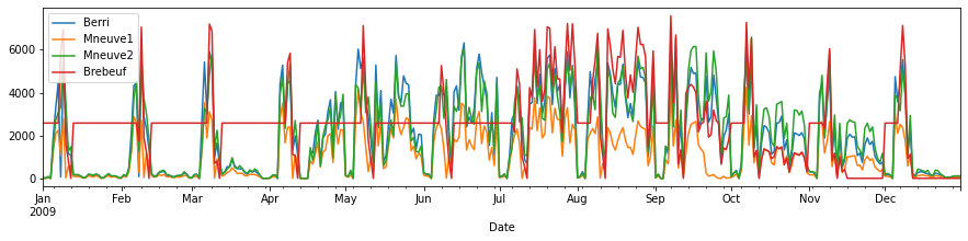
# Graficar usando plot, se grafican las variables numéricas, donde el eje X corresponde al índice con las fechas
d.plot(figsize=(15,3))

<AxesSubplot:xlabel='Date'>

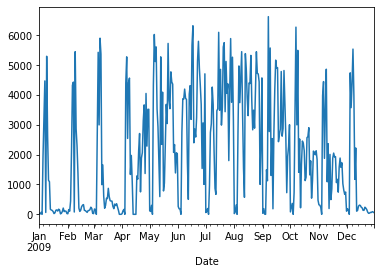
# Graficas sólo una columna (Berri)
d.Berri.plot()

<AxesSubplot:xlabel='Date'>

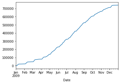
# Graficas la columna Berri de forma suma acumulada
d.Berri.cumsum().plot()

<matplotlib.axes._subplots.AxesSubplot at 0x7f894e1c47d0>

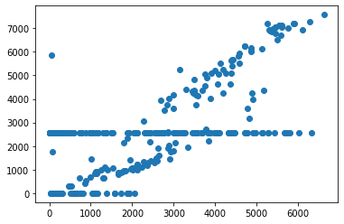
# Graficar puntos para datos de dos columnas
plt.scatter(d.Berri, d.Brebeuf)

<matplotlib.collections.PathCollection at 0x7f484cf3f7f0>

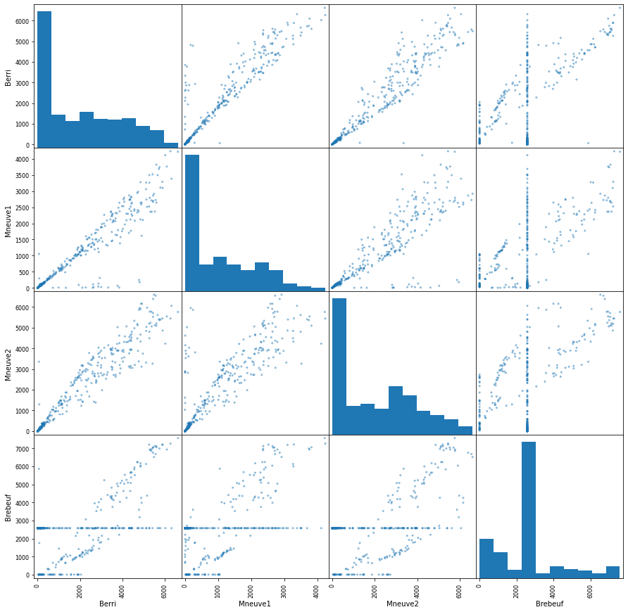
# Graficar puntos todas las columnas contra todas, la diagonal principal corresponde al histograma
pd.plotting.scatter_matrix(d, figsize=(15,15))

array([[<AxesSubplot:xlabel='Berri', ylabel='Berri'>,
        <AxesSubplot:xlabel='Mneuve1', ylabel='Berri'>,
        <AxesSubplot:xlabel='Mneuve2', ylabel='Berri'>,
        <AxesSubplot:xlabel='Brebeuf', ylabel='Berri'>],
       [<AxesSubplot:xlabel='Berri', ylabel='Mneuve1'>,
        <AxesSubplot:xlabel='Mneuve1', ylabel='Mneuve1'>,
        <AxesSubplot:xlabel='Mneuve2', ylabel='Mneuve1'>,
        <AxesSubplot:xlabel='Brebeuf', ylabel='Mneuve1'>],
       [<AxesSubplot:xlabel='Berri', ylabel='Mneuve2'>,
        <AxesSubplot:xlabel='Mneuve1', ylabel='Mneuve2'>,
        <AxesSubplot:xlabel='Mneuve2', ylabel='Mneuve2'>,
        <AxesSubplot:xlabel='Brebeuf', ylabel='Mneuve2'>],
       [<AxesSubplot:xlabel='Berri', ylabel='Brebeuf'>,
        <AxesSubplot:xlabel='Mneuve1', ylabel='Brebeuf'>,
        <AxesSubplot:xlabel='Mneuve2', ylabel='Brebeuf'>,
        <AxesSubplot:xlabel='Brebeuf', ylabel='Brebeuf'>]], dtype=object)

Agrupamiento

# Dado que los índices corresponden a fechas, obtener solamente el mes de la fecha 
for i in d.index:
    print(i.month)

1
1
1
1
1
1
1
1
1
1
1
1
1
1
1
1
1
1
1
1
1
1
1
1
1
1
1
1
1
1
1
2
2
2
2
2
2
2
2
2
2
2
2
2
2
2
2
2
2
2
2
2
2
2
2
2
2
2
2
3
3
3
3
3
3
3
3
3
3
3
3
3
3
3
3
3
3
3
3
3
3
3
3
3
3
3
3
3
3
3
4
4
4
4
4
4
4
4
4
4
4
4
4
4
4
4
4
4
4
4
4
4
4
4
4
4
4
4
4
4
5
5
5
5
5
5
5
5
5
5
5
5
5
5
5
5
5
5
5
5
5
5
5
5
5
5
5
5
5
5
5
6
6
6
6
6
6
6
6
6
6
6
6
6
6
6
6
6
6
6
6
6
6
6
6
6
6
6
6
6
6
7
7
7
7
7
7
7
7
7
7
7
7
7
7
7
7
7
7
7
7
7
7
7
7
7
7
7
7
7
7
7
8
8
8
8
8
8
8
8
8
8
8
8
8
8
8
8
8
8
8
8
8
8
8
8
8
8
8
8
8
8
8
9
9
9
9
9
9
9
9
9
9
9
9
9
9
9
9
9
9
9
9
9
9
9
9
9
9
9
9
9
9
10
10
10
10
10
10
10
10
10
10
10
10
10
10
10
10
10
10
10
10
10
10
10
10
10
10
10
10
10
10
10
11
11
11
11
11
11
11
11
11
11
11
11
11
11
11
11
11
11
11
11
11
11
11
11
11
11
11
11
11
11
12
12
12
12
12
12
12
12
12
12
12
12
12
12
12
12
12
12
12
12
12
12
12
12
12
12
12
12
12
12
12

# Crear nueva columna con el mes, que se extrae de los indices
d["month"] = [i.month for i in d.index]
d.head(100)

	Berri	Mneuve1	Mneuve2	Brebeuf	month
Date
2009-01-01	29	20	35	2576.359551	1
2009-01-02	14	2	2	2576.359551	1
2009-01-03	67	30	80	2576.359551	1
2009-01-04	0	0	0	2576.359551	1
2009-01-05	1925	1256	1501	2576.359551	1
...	...	...	...	...	...
2009-04-06	5278	3499	4795	2576.359551	4
2009-04-07	2544	1653	2325	2576.359551	4
2009-04-08	4417	2382	4350	5384.000000	4
2009-04-09	4566	2393	5327	5837.000000	4
2009-04-10	1336	0	1620	1116.000000	4

100 rows × 5 columns

# Agrupar por el mes (columna creada), los valores máximos
d.groupby("month").max()

	Berri	Mneuve1	Mneuve2	Brebeuf
month
1	5298	2796	5765	6939.0
2	5451	2868	5517	7052.0
3	5904	3523	5762	7194.0
4	5278	3499	5327	5837.0
5	6028	4120	5397	7121.0
6	6320	3499	6047	5259.0
7	6100	3825	5536	7219.0
8	5452	2865	6379	7044.0
9	6626	4227	6535	7575.0
10	6274	4242	6587	7268.0
11	4864	2648	5895	6044.0
12	5538	2983	5107	7127.0

# Agrupar por el mes (columna creada), el conteo de datos
d.groupby("month").count()

	Berri	Mneuve1	Mneuve2	Brebeuf
month
1	31	31	31	31
2	28	28	28	28
3	31	31	31	31
4	30	30	30	30
5	31	31	31	31
6	30	30	30	30
7	31	31	31	31
8	31	31	31	31
9	30	30	30	30
10	31	31	31	31
11	30	30	30	30
12	31	31	31	31