Ejemplo de ciencia de datos

Lectura del dataset

# Ruta donde se encuentran los datos en Github
path = "https://raw.githubusercontent.com/BioAITeamLearning/IntroPython_2024_01_UAI/main/Data/"

# Leer el dataset
import pandas as pd
df = pd.read_csv(path+"BDParkinson_Prediction.csv")

df

	VAR1	VAR2	VAR3	VAR4	VAR5	VAR6	CLASS
0	0.624731	0.135424	0.000000	0.675282	0.182203	0.962960	Class_1
1	0.647223	0.136211	0.000000	0.679511	0.195903	0.987387	Class_1
2	0.706352	0.187593	0.000000	0.632989	0.244884	0.991182	Class_1
3	0.680291	0.192076	0.000000	0.651786	0.233528	0.991857	Class_1
4	0.660104	0.161131	0.000000	0.677162	0.209531	0.991066	Class_1
...	...	...	...	...	...	...	...
495	0.712586	0.219776	0.510939	0.593045	0.268087	0.092055	Class_4
496	0.686058	0.224004	0.518661	0.600564	0.253298	0.093827	Class_4
497	0.698661	0.216604	0.505791	0.591165	0.241696	0.090734	Class_4
498	0.714926	0.222613	0.562420	0.587406	0.271037	0.093245	Class_4
499	0.698690	0.219577	0.541828	0.583647	0.258280	0.091973	Class_4

500 rows × 7 columns

División en datos de entrenamiento y testing

# Obtener las features
features = df.drop(['CLASS'], axis=1)
features.head()

	VAR1	VAR2	VAR3	VAR4	VAR5	VAR6
0	0.624731	0.135424	0.0	0.675282	0.182203	0.962960
1	0.647223	0.136211	0.0	0.679511	0.195903	0.987387
2	0.706352	0.187593	0.0	0.632989	0.244884	0.991182
3	0.680291	0.192076	0.0	0.651786	0.233528	0.991857
4	0.660104	0.161131	0.0	0.677162	0.209531	0.991066

# Obtener los labels
labels = df['CLASS']
labels.head()

0    Class_1
1    Class_1
2    Class_1
3    Class_1
4    Class_1
Name: CLASS, dtype: object

# Separación de la data, con un 20% para testing, y 80% para entrenamiento
from sklearn.model_selection import train_test_split
X_train, X_test, y_train, y_test = train_test_split(features, labels,
                                                    test_size=0.20, random_state=1, stratify=labels)

# Verificacion de la cantidad de datos para entrenamiento y para testing
import numpy as np
print("y_train labels unique:",np.unique(y_train, return_counts=True))
print("y_test labels unique: ",np.unique(y_test, return_counts=True))

y_train labels unique: (array(['Class2', 'Class_1', 'Class_3', 'Class_4'], dtype=object), array([100, 100, 100, 100]))
y_test labels unique:  (array(['Class2', 'Class_1', 'Class_3', 'Class_4'], dtype=object), array([25, 25, 25, 25]))

Aprendizaje supervisado

Clasificación

# Cargamos el modelo KNN sin entrenar
from sklearn.neighbors import KNeighborsClassifier
model_KNN = KNeighborsClassifier(n_neighbors=3)
# Entrenamos el modelo KNN
model_KNN.fit(X_train, y_train)
# Obtenemos la métrica lograda
model_KNN.score(X_test, y_test)

1.0

df

	VAR1	VAR2	VAR3	VAR4	VAR5	VAR6	CLASS
0	0.624731	0.135424	0.000000	0.675282	0.182203	0.962960	Class_1
1	0.647223	0.136211	0.000000	0.679511	0.195903	0.987387	Class_1
2	0.706352	0.187593	0.000000	0.632989	0.244884	0.991182	Class_1
3	0.680291	0.192076	0.000000	0.651786	0.233528	0.991857	Class_1
4	0.660104	0.161131	0.000000	0.677162	0.209531	0.991066	Class_1
...	...	...	...	...	...	...	...
495	0.712586	0.219776	0.510939	0.593045	0.268087	0.092055	Class_4
496	0.686058	0.224004	0.518661	0.600564	0.253298	0.093827	Class_4
497	0.698661	0.216604	0.505791	0.591165	0.241696	0.090734	Class_4
498	0.714926	0.222613	0.562420	0.587406	0.271037	0.093245	Class_4
499	0.698690	0.219577	0.541828	0.583647	0.258280	0.091973	Class_4

500 rows × 7 columns

model_KNN.predict([[0.712586	,0.219776	,0.510939,	0.593045,	0.268087,	0.092055]])

/usr/local/lib/python3.10/dist-packages/sklearn/base.py:439: UserWarning: X does not have valid feature names, but KNeighborsClassifier was fitted with feature names
  warnings.warn(

array(['Class_4'], dtype=object)

y_test

2      Class_1
92     Class_1
255    Class_3
105    Class_1
468    Class_4
        ...   
316    Class_3
126     Class2
280    Class_3
118    Class_1
318    Class_3
Name: CLASS, Length: 100, dtype: object

# Metricas: matriz de confusión y reporte de clasificación
from sklearn.metrics import confusion_matrix
from sklearn.metrics import classification_report

# Predecir y obtener la matriz de confusión
y_pred=model_KNN.predict(X_test)
print(confusion_matrix(y_test,y_pred))
print(classification_report(y_test,y_pred))

[[25  0  0  0]
 [ 0 25  0  0]
 [ 0  0 25  0]
 [ 0  0  0 25]]
              precision    recall  f1-score   support

      Class2       1.00      1.00      1.00        25
     Class_1       1.00      1.00      1.00        25
     Class_3       1.00      1.00      1.00        25
     Class_4       1.00      1.00      1.00        25

    accuracy                           1.00       100
   macro avg       1.00      1.00      1.00       100
weighted avg       1.00      1.00      1.00       100

# Crear los modelos

from sklearn.tree import DecisionTreeClassifier
model_DT  = DecisionTreeClassifier(random_state=0)

from sklearn.ensemble import BaggingClassifier
model_B   = BaggingClassifier(random_state=0)

from sklearn.ensemble import RandomForestClassifier
model_RF  = RandomForestClassifier(random_state=0)

from sklearn.ensemble import AdaBoostClassifier
model_AB  = AdaBoostClassifier(random_state=0)

from sklearn.svm import SVC
model_SVM = SVC(random_state=0)

from sklearn.ensemble import ExtraTreesClassifier
model_ET  = ExtraTreesClassifier(random_state=0)

from xgboost import XGBClassifier
model_XGB = XGBClassifier(random_state=0)

from sklearn.linear_model import LogisticRegression
model_LR  = LogisticRegression(random_state=0, max_iter=200)

from sklearn.ensemble import GradientBoostingClassifier
model_GB  = GradientBoostingClassifier(random_state=0)

from sklearn.discriminant_analysis import QuadraticDiscriminantAnalysis
model_QDA = QuadraticDiscriminantAnalysis()

from sklearn.discriminant_analysis import LinearDiscriminantAnalysis
model_LDA = LinearDiscriminantAnalysis()

from sklearn.naive_bayes import GaussianNB
model_GNB = GaussianNB()

# Ajustar los modelos a la data de entrenamiento
model_DT.fit(X_train, y_train)
model_B.fit(X_train, y_train)
model_RF.fit(X_train, y_train)
model_AB.fit(X_train, y_train)
model_SVM.fit(X_train, y_train)
model_ET.fit(X_train, y_train)
#model_XGB.fit(X_train, y_train)
model_LR.fit(X_train, y_train)
model_GB.fit(X_train, y_train)
model_QDA.fit(X_train, y_train)
model_LDA.fit(X_train, y_train)
model_GNB.fit(X_train, y_train)

GaussianNB()

In a Jupyter environment, please rerun this cell to show the HTML representation or trust the notebook.
On GitHub, the HTML representation is unable to render, please try loading this page with nbviewer.org.

# Predecir y obtener el accuracy
print("DT, Accuracy: ", model_DT.score(X_test, y_test))
print("B, Accuracy: ",  model_B.score(X_test, y_test))
print("RF, Accuracy: ", model_RF.score(X_test, y_test))
print("AB, Accuracy: ", model_AB.score(X_test, y_test))
print("SVM, Accuracy: ",model_SVM.score(X_test, y_test))
print("ET, Accuracy: ", model_ET.score(X_test, y_test))
#print("XGB, Accuracy: ",model_XGB.score(X_test, y_test))
print("LR, Accuracy: ", model_LR.score(X_test, y_test))
print("GB, Accuracy: ", model_GB.score(X_test, y_test))
print("QDA, Accuracy: ",model_QDA.score(X_test, y_test))
print("LDA, Accuracy: ",model_LDA.score(X_test, y_test))
print("GNB, Accuracy: ",model_GNB.score(X_test, y_test))

DT, Accuracy:  0.99
B, Accuracy:  0.99
RF, Accuracy:  0.97
AB, Accuracy:  0.74
SVM, Accuracy:  0.97
ET, Accuracy:  0.99
LR, Accuracy:  0.97
GB, Accuracy:  0.98
QDA, Accuracy:  1.0
LDA, Accuracy:  1.0
GNB, Accuracy:  0.98

Regresión

# Seleccionando datos para hacer regresión
## Train
X_train_reg = X_train.drop(['VAR5'], axis=1)
y_train_reg = X_train['VAR5']

## Test
X_test_reg = X_test.drop(['VAR5'], axis=1)
y_test_reg = X_test['VAR5']

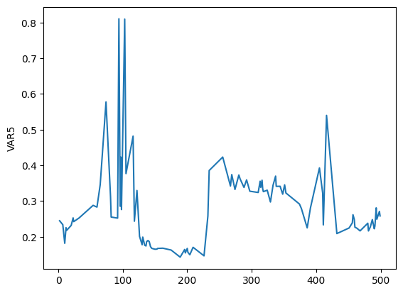
import seaborn as sns
# Gráfica de la variable objetivo
sns.lineplot(data=y_test_reg)

<Axes: ylabel='VAR5'>

from sklearn.neighbors import KNeighborsRegressor

# Cargamos el modelo KNN sin entrenar
model_KNNr = KNeighborsRegressor(n_neighbors=3)

# Entrenamos el modelo KNN
model_KNNr.fit(X_train_reg, y_train_reg)

# Obtenemos la métrica lograda
model_KNNr.score(X_test_reg, y_test_reg)

0.9631421177334887

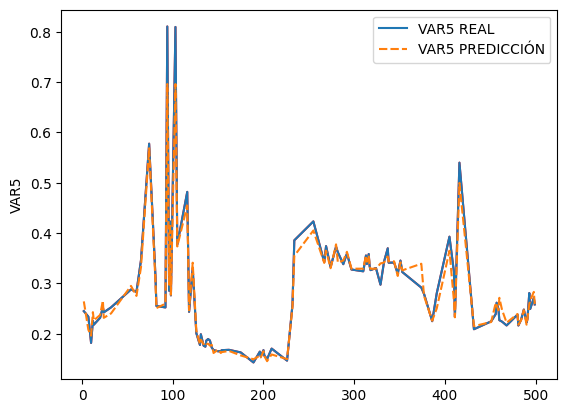
# Gráfica de la variable objetivo real
sns.lineplot(data=y_test_reg,c='r')

# Gráfica de la variable objetivo predicción
y_pred_reg = model_KNNr.predict(X_test_reg)
y_pred_reg = pd.DataFrame(y_pred_reg).set_index(y_test_reg.index)

# Creando un dataframe 2 columnas con variable real y la predicción
df_test_real_pred = pd.concat([y_test_reg,y_pred_reg],axis=1)
df_test_real_pred.rename(columns={'VAR5':'VAR5 REAL',
                        0:'VAR5 PREDICCIÓN'},inplace=True)

sns.lineplot(data=df_test_real_pred)

<Axes: ylabel='VAR5'>

# Crear los modelos
from sklearn.tree import DecisionTreeRegressor
model_DTr  = DecisionTreeRegressor()

from sklearn.ensemble import BaggingRegressor
model_Br   = BaggingRegressor()

from sklearn.ensemble import RandomForestRegressor
model_RFr  = RandomForestRegressor()

from sklearn.ensemble import AdaBoostRegressor
model_ABr  = AdaBoostRegressor()

from sklearn.svm import SVR
model_SVMr = SVR()

from sklearn.ensemble import ExtraTreesRegressor
model_ETr  = ExtraTreesRegressor()

from xgboost import XGBRegressor
model_XGBr = XGBRegressor()

from sklearn.linear_model import LinearRegression
model_Lr   = LinearRegression()

from sklearn.ensemble import GradientBoostingRegressor
model_GBr  = GradientBoostingRegressor()

# Ajustar los modelos a la data de entrenamiento
model_DTr.fit(X_train_reg, y_train_reg)
model_Br.fit(X_train_reg, y_train_reg)
model_RFr.fit(X_train_reg, y_train_reg)
model_ABr.fit(X_train_reg, y_train_reg)
model_SVMr.fit(X_train_reg, y_train_reg)
model_ETr.fit(X_train_reg, y_train_reg)
model_XGBr.fit(X_train_reg, y_train_reg)
model_Lr.fit(X_train_reg, y_train_reg)
model_GBr.fit(X_train_reg, y_train_reg)

GradientBoostingRegressor()

In a Jupyter environment, please rerun this cell to show the HTML representation or trust the notebook.
On GitHub, the HTML representation is unable to render, please try loading this page with nbviewer.org.

# Predecir y obtener el coeficiente de determinación
print("DTr: ",model_DTr.score(X_test_reg, y_test_reg))
print("Br: ",model_Br.score(X_test_reg, y_test_reg))
print("RFr: ",model_RFr.score(X_test_reg, y_test_reg))
print("ABr: ",model_ABr.score(X_test_reg, y_test_reg))
print("SVMr: ",model_SVMr.score(X_test_reg, y_test_reg))
print("ETr: ",model_ETr.score(X_test_reg, y_test_reg))
print("XGBr: ",model_XGBr.score(X_test_reg, y_test_reg))
print("Lr: ",model_Lr.score(X_test_reg, y_test_reg))
print("GBr: ",model_GBr.score(X_test_reg, y_test_reg))

DTr:  0.9333939473701152
Br:  0.9521755430796952
RFr:  0.9463222743232533
ABr:  0.9327701413351718
SVMr:  0.5280872992079053
ETr:  0.9637670215745208
XGBr:  0.948858853029048
Lr:  0.7546713332247559
GBr:  0.9468085388548643

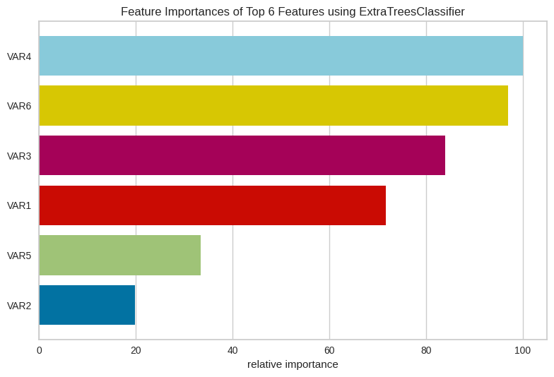
Importancia de características

# Definir el algoritmo de ML
from sklearn.ensemble import ExtraTreesClassifier
model = ExtraTreesClassifier()
model.fit(X_train, y_train)


# Importancia de características
from yellowbrick.model_selection import FeatureImportances
# Mostrar la importancia de características
viz = FeatureImportances(model, topn=6)
viz.fit(X_train, y_train)
viz.show()

/usr/local/lib/python3.10/dist-packages/sklearn/base.py:439: UserWarning: X does not have valid feature names, but ExtraTreesClassifier was fitted with feature names
  warnings.warn(

<Axes: title={'center': 'Feature Importances of Top 6 Features using ExtraTreesClassifier'}, xlabel='relative importance'>

feature_importances=pd.DataFrame({'features':features.columns,'feature_importance':model.feature_importances_})
feature_importances.sort_values('feature_importance',ascending=False)[:6]

	features	feature_importance
3	VAR4	0.246367
5	VAR6	0.238958
2	VAR3	0.206822
0	VAR1	0.176625
4	VAR5	0.082190
1	VAR2	0.049038

model = SVC(kernel="linear",random_state=0)
model.fit(X_train, y_train)
feature_importance=pd.DataFrame({'feature':list(features.columns),'feature_importance':[abs(i) for i in model.coef_[0]]})
feature_importance.sort_values('feature_importance',ascending=False)[:20]

	feature	feature_importance
5	VAR6	1.566236
2	VAR3	1.081330
1	VAR2	0.739577
3	VAR4	0.237416
4	VAR5	0.214015
0	VAR1	0.051399

Reto: Clasifiquemos nuestra primer base de datos

import pandas as pd
from sklearn.datasets import load_iris

data = load_iris()
caracteristicas = pd.DataFrame(data=data.data,columns=data.feature_names)
resultados = data.target
caracteristicas.head()

	sepal length (cm)	sepal width (cm)	petal length (cm)	petal width (cm)
0	5.1	3.5	1.4	0.2
1	4.9	3.0	1.4	0.2
2	4.7	3.2	1.3	0.2
3	4.6	3.1	1.5	0.2
4	5.0	3.6	1.4	0.2

## IMPLEMENTA UN MODELO DE ML PARA CLASIFICAR ESTA BASE DE DATOS EN CADA UNA DE LAS CLASES.