Ejemplo de ciencia de datos

Lectura del dataset

# Ruta donde se encuentran los datos en Github
path_datos = "https://raw.githubusercontent.com/BioAITeamLearning/IntroPython_2024_01_UAI/main/Data/"

import pandas as pd
# Leer el dataset
df = pd.read_csv(path_datos+"/wisc_bc_data.csv")
df2 = pd.read_csv(path_datos+"/BDParkinson_Prediction.csv")

# Mostrar el dataframe
df.head(20)

	id	diagnosis	radius_mean	texture_mean	perimeter_mean	area_mean	smoothness_mean	compactness_mean	concavity_mean	concave points_mean	...	radius_worst	texture_worst	perimeter_worst	area_worst	smoothness_worst	compactness_worst	concavity_worst	concave points_worst	symmetry_worst	fractal_dimension_worst
0	842302	M	17.99	10.38	122.80	1001.0	0.11840	0.27760	0.30010	0.14710	...	25.38	17.33	184.60	2019.0	0.1622	0.6656	0.7119	0.26540	0.4601	0.11890
1	842517	M	20.57	17.77	132.90	1326.0	0.08474	0.07864	0.08690	0.07017	...	24.99	23.41	158.80	1956.0	0.1238	0.1866	0.2416	0.18600	0.2750	0.08902
2	84300903	M	19.69	21.25	130.00	1203.0	0.10960	0.15990	0.19740	0.12790	...	23.57	25.53	152.50	1709.0	0.1444	0.4245	0.4504	0.24300	0.3613	0.08758
3	84348301	M	11.42	20.38	77.58	386.1	0.14250	0.28390	0.24140	0.10520	...	14.91	26.50	98.87	567.7	0.2098	0.8663	0.6869	0.25750	0.6638	0.17300
4	84358402	M	20.29	14.34	135.10	1297.0	0.10030	0.13280	0.19800	0.10430	...	22.54	16.67	152.20	1575.0	0.1374	0.2050	0.4000	0.16250	0.2364	0.07678
5	843786	M	12.45	15.70	82.57	477.1	0.12780	0.17000	0.15780	0.08089	...	15.47	23.75	103.40	741.6	0.1791	0.5249	0.5355	0.17410	0.3985	0.12440
6	844359	M	18.25	19.98	119.60	1040.0	0.09463	0.10900	0.11270	0.07400	...	22.88	27.66	153.20	1606.0	0.1442	0.2576	0.3784	0.19320	0.3063	0.08368
7	84458202	M	13.71	20.83	90.20	577.9	0.11890	0.16450	0.09366	0.05985	...	17.06	28.14	110.60	897.0	0.1654	0.3682	0.2678	0.15560	0.3196	0.11510
8	844981	M	13.00	21.82	87.50	519.8	0.12730	0.19320	0.18590	0.09353	...	15.49	30.73	106.20	739.3	0.1703	0.5401	0.5390	0.20600	0.4378	0.10720
9	84501001	M	12.46	24.04	83.97	475.9	0.11860	0.23960	0.22730	0.08543	...	15.09	40.68	97.65	711.4	0.1853	1.0580	1.1050	0.22100	0.4366	0.20750
10	845636	M	16.02	23.24	102.70	797.8	0.08206	0.06669	0.03299	0.03323	...	19.19	33.88	123.80	1150.0	0.1181	0.1551	0.1459	0.09975	0.2948	0.08452
11	84610002	M	15.78	17.89	103.60	781.0	0.09710	0.12920	0.09954	0.06606	...	20.42	27.28	136.50	1299.0	0.1396	0.5609	0.3965	0.18100	0.3792	0.10480
12	846226	M	19.17	24.80	132.40	1123.0	0.09740	0.24580	0.20650	0.11180	...	20.96	29.94	151.70	1332.0	0.1037	0.3903	0.3639	0.17670	0.3176	0.10230
13	846381	M	15.85	23.95	103.70	782.7	0.08401	0.10020	0.09938	0.05364	...	16.84	27.66	112.00	876.5	0.1131	0.1924	0.2322	0.11190	0.2809	0.06287
14	84667401	M	13.73	22.61	93.60	578.3	0.11310	0.22930	0.21280	0.08025	...	15.03	32.01	108.80	697.7	0.1651	0.7725	0.6943	0.22080	0.3596	0.14310
15	84799002	M	14.54	27.54	96.73	658.8	0.11390	0.15950	0.16390	0.07364	...	17.46	37.13	124.10	943.2	0.1678	0.6577	0.7026	0.17120	0.4218	0.13410
16	848406	M	14.68	20.13	94.74	684.5	0.09867	0.07200	0.07395	0.05259	...	19.07	30.88	123.40	1138.0	0.1464	0.1871	0.2914	0.16090	0.3029	0.08216
17	84862001	M	16.13	20.68	108.10	798.8	0.11700	0.20220	0.17220	0.10280	...	20.96	31.48	136.80	1315.0	0.1789	0.4233	0.4784	0.20730	0.3706	0.11420
18	849014	M	19.81	22.15	130.00	1260.0	0.09831	0.10270	0.14790	0.09498	...	27.32	30.88	186.80	2398.0	0.1512	0.3150	0.5372	0.23880	0.2768	0.07615
19	8510426	B	13.54	14.36	87.46	566.3	0.09779	0.08129	0.06664	0.04781	...	15.11	19.26	99.70	711.2	0.1440	0.1773	0.2390	0.12880	0.2977	0.07259

20 rows × 32 columns

# Mostrar todas las columnas del dataframe
pd.options.display.max_columns = None
# Mostrar el dataframe ya con todas las columnas
df.head(5)

	id	diagnosis	radius_mean	texture_mean	perimeter_mean	area_mean	smoothness_mean	compactness_mean	concavity_mean	concave points_mean	symmetry_mean	fractal_dimension_mean	radius_se	texture_se	perimeter_se	area_se	smoothness_se	compactness_se	concavity_se	concave points_se	symmetry_se	fractal_dimension_se	radius_worst	texture_worst	perimeter_worst	area_worst	smoothness_worst	compactness_worst	concavity_worst	concave points_worst	symmetry_worst	fractal_dimension_worst
0	842302	M	17.99	10.38	122.80	1001.0	0.11840	0.27760	0.3001	0.14710	0.2419	0.07871	1.0950	0.9053	8.589	153.40	0.006399	0.04904	0.05373	0.01587	0.03003	0.006193	25.38	17.33	184.60	2019.0	0.1622	0.6656	0.7119	0.2654	0.4601	0.11890
1	842517	M	20.57	17.77	132.90	1326.0	0.08474	0.07864	0.0869	0.07017	0.1812	0.05667	0.5435	0.7339	3.398	74.08	0.005225	0.01308	0.01860	0.01340	0.01389	0.003532	24.99	23.41	158.80	1956.0	0.1238	0.1866	0.2416	0.1860	0.2750	0.08902
2	84300903	M	19.69	21.25	130.00	1203.0	0.10960	0.15990	0.1974	0.12790	0.2069	0.05999	0.7456	0.7869	4.585	94.03	0.006150	0.04006	0.03832	0.02058	0.02250	0.004571	23.57	25.53	152.50	1709.0	0.1444	0.4245	0.4504	0.2430	0.3613	0.08758
3	84348301	M	11.42	20.38	77.58	386.1	0.14250	0.28390	0.2414	0.10520	0.2597	0.09744	0.4956	1.1560	3.445	27.23	0.009110	0.07458	0.05661	0.01867	0.05963	0.009208	14.91	26.50	98.87	567.7	0.2098	0.8663	0.6869	0.2575	0.6638	0.17300
4	84358402	M	20.29	14.34	135.10	1297.0	0.10030	0.13280	0.1980	0.10430	0.1809	0.05883	0.7572	0.7813	5.438	94.44	0.011490	0.02461	0.05688	0.01885	0.01756	0.005115	22.54	16.67	152.20	1575.0	0.1374	0.2050	0.4000	0.1625	0.2364	0.07678

# Mostrar nombres de las columnas
list(df.columns.values)

['id',
 'diagnosis',
 'radius_mean',
 'texture_mean',
 'perimeter_mean',
 'area_mean',
 'smoothness_mean',
 'compactness_mean',
 'concavity_mean',
 'concave points_mean',
 'symmetry_mean',
 'fractal_dimension_mean',
 'radius_se',
 'texture_se',
 'perimeter_se',
 'area_se',
 'smoothness_se',
 'compactness_se',
 'concavity_se',
 'concave points_se',
 'symmetry_se',
 'fractal_dimension_se',
 'radius_worst',
 'texture_worst',
 'perimeter_worst',
 'area_worst',
 'smoothness_worst',
 'compactness_worst',
 'concavity_worst',
 'concave points_worst',
 'symmetry_worst',
 'fractal_dimension_worst']

Eliminar columnas innecesarias del dataset

# Eliminar la columna de identificación, esta no se puede usar como feature
df = df.drop(['id'], axis=1)

# Mostramos el df sin la identificación
df.head()

	diagnosis	radius_mean	texture_mean	perimeter_mean	area_mean	smoothness_mean	compactness_mean	concavity_mean	concave points_mean	symmetry_mean	fractal_dimension_mean	radius_se	texture_se	perimeter_se	area_se	smoothness_se	compactness_se	concavity_se	concave points_se	symmetry_se	fractal_dimension_se	radius_worst	texture_worst	perimeter_worst	area_worst	smoothness_worst	compactness_worst	concavity_worst	concave points_worst	symmetry_worst	fractal_dimension_worst
0	M	17.99	10.38	122.80	1001.0	0.11840	0.27760	0.3001	0.14710	0.2419	0.07871	1.0950	0.9053	8.589	153.40	0.006399	0.04904	0.05373	0.01587	0.03003	0.006193	25.38	17.33	184.60	2019.0	0.1622	0.6656	0.7119	0.2654	0.4601	0.11890
1	M	20.57	17.77	132.90	1326.0	0.08474	0.07864	0.0869	0.07017	0.1812	0.05667	0.5435	0.7339	3.398	74.08	0.005225	0.01308	0.01860	0.01340	0.01389	0.003532	24.99	23.41	158.80	1956.0	0.1238	0.1866	0.2416	0.1860	0.2750	0.08902
2	M	19.69	21.25	130.00	1203.0	0.10960	0.15990	0.1974	0.12790	0.2069	0.05999	0.7456	0.7869	4.585	94.03	0.006150	0.04006	0.03832	0.02058	0.02250	0.004571	23.57	25.53	152.50	1709.0	0.1444	0.4245	0.4504	0.2430	0.3613	0.08758
3	M	11.42	20.38	77.58	386.1	0.14250	0.28390	0.2414	0.10520	0.2597	0.09744	0.4956	1.1560	3.445	27.23	0.009110	0.07458	0.05661	0.01867	0.05963	0.009208	14.91	26.50	98.87	567.7	0.2098	0.8663	0.6869	0.2575	0.6638	0.17300
4	M	20.29	14.34	135.10	1297.0	0.10030	0.13280	0.1980	0.10430	0.1809	0.05883	0.7572	0.7813	5.438	94.44	0.011490	0.02461	0.05688	0.01885	0.01756	0.005115	22.54	16.67	152.20	1575.0	0.1374	0.2050	0.4000	0.1625	0.2364	0.07678

Análisis exploratorio de datos (Exploratory data analysis - EDA)

# Cantidad de clases
print(f'Número de clases {len(df["diagnosis"].value_counts())}')

Número de clases 2

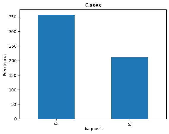
# Frecuencia por clase
print(df["diagnosis"].value_counts())

ax = df['diagnosis'].value_counts().plot(kind='bar')
ax.set_title('Clases')
ax.set_ylabel('Frecuencia')

diagnosis
B    357
M    212
Name: count, dtype: int64

Text(0, 0.5, 'Frecuencia')

# Cuenta de datos en las features, se puede verificar que no haya features con valores nulos
df.groupby("diagnosis").count()

	radius_mean	texture_mean	perimeter_mean	area_mean	smoothness_mean	compactness_mean	concavity_mean	concave points_mean	symmetry_mean	fractal_dimension_mean	radius_se	texture_se	perimeter_se	area_se	smoothness_se	compactness_se	concavity_se	concave points_se	symmetry_se	fractal_dimension_se	radius_worst	texture_worst	perimeter_worst	area_worst	smoothness_worst	compactness_worst	concavity_worst	concave points_worst	symmetry_worst	fractal_dimension_worst
diagnosis
B	357	357	357	357	357	357	357	357	357	357	357	357	357	357	357	357	357	357	357	357	357	357	357	357	357	357	357	357	357	357
M	212	212	212	212	212	212	212	212	212	212	212	212	212	212	212	212	212	212	212	212	212	212	212	212	212	212	212	212	212	212

# Renombrar features con espacios en los nombres
df.rename(columns={'concave points_mean':'concave_points_mean',
                   'concave points_se':'concave_points_se',
                   'concave points_worst':'concave_points_worst'},inplace=True)

# Nombre de las features, conteo de cantidades, verificación de valores nulos, ver tipo de dato de cada feature
df.info()

<class 'pandas.core.frame.DataFrame'>
RangeIndex: 569 entries, 0 to 568
Data columns (total 31 columns):
 #   Column                   Non-Null Count  Dtype  
---  ------                   --------------  -----  
 0   diagnosis                569 non-null    object 
 1   radius_mean              569 non-null    float64
 2   texture_mean             569 non-null    float64
 3   perimeter_mean           569 non-null    float64
 4   area_mean                569 non-null    float64
 5   smoothness_mean          569 non-null    float64
 6   compactness_mean         569 non-null    float64
 7   concavity_mean           569 non-null    float64
 8   concave_points_mean      569 non-null    float64
 9   symmetry_mean            569 non-null    float64
 10  fractal_dimension_mean   569 non-null    float64
 11  radius_se                569 non-null    float64
 12  texture_se               569 non-null    float64
 13  perimeter_se             569 non-null    float64
 14  area_se                  569 non-null    float64
 15  smoothness_se            569 non-null    float64
 16  compactness_se           569 non-null    float64
 17  concavity_se             569 non-null    float64
 18  concave_points_se        569 non-null    float64
 19  symmetry_se              569 non-null    float64
 20  fractal_dimension_se     569 non-null    float64
 21  radius_worst             569 non-null    float64
 22  texture_worst            569 non-null    float64
 23  perimeter_worst          569 non-null    float64
 24  area_worst               569 non-null    float64
 25  smoothness_worst         569 non-null    float64
 26  compactness_worst        569 non-null    float64
 27  concavity_worst          569 non-null    float64
 28  concave_points_worst     569 non-null    float64
 29  symmetry_worst           569 non-null    float64
 30  fractal_dimension_worst  569 non-null    float64
dtypes: float64(30), object(1)
memory usage: 137.9+ KB

# Estadísticas básicas en las features
# Cuenta de datos, media, desviación estandar, valor mínimo, cuartiles, y valor máximo
df.describe()

	radius_mean	texture_mean	perimeter_mean	area_mean	smoothness_mean	compactness_mean	concavity_mean	concave_points_mean	symmetry_mean	fractal_dimension_mean	radius_se	texture_se	perimeter_se	area_se	smoothness_se	compactness_se	concavity_se	concave_points_se	symmetry_se	fractal_dimension_se	radius_worst	texture_worst	perimeter_worst	area_worst	smoothness_worst	compactness_worst	concavity_worst	concave_points_worst	symmetry_worst	fractal_dimension_worst
count	569.000000	569.000000	569.000000	569.000000	569.000000	569.000000	569.000000	569.000000	569.000000	569.000000	569.000000	569.000000	569.000000	569.000000	569.000000	569.000000	569.000000	569.000000	569.000000	569.000000	569.000000	569.000000	569.000000	569.000000	569.000000	569.000000	569.000000	569.000000	569.000000	569.000000
mean	14.127292	19.289649	91.969033	654.889104	0.096360	0.104341	0.088799	0.048919	0.181162	0.062798	0.405172	1.216853	2.866059	40.337079	0.007041	0.025478	0.031894	0.011796	0.020542	0.003795	16.269190	25.677223	107.261213	880.583128	0.132369	0.254265	0.272188	0.114606	0.290076	0.083946
std	3.524049	4.301036	24.298981	351.914129	0.014064	0.052813	0.079720	0.038803	0.027414	0.007060	0.277313	0.551648	2.021855	45.491006	0.003003	0.017908	0.030186	0.006170	0.008266	0.002646	4.833242	6.146258	33.602542	569.356993	0.022832	0.157336	0.208624	0.065732	0.061867	0.018061
min	6.981000	9.710000	43.790000	143.500000	0.052630	0.019380	0.000000	0.000000	0.106000	0.049960	0.111500	0.360200	0.757000	6.802000	0.001713	0.002252	0.000000	0.000000	0.007882	0.000895	7.930000	12.020000	50.410000	185.200000	0.071170	0.027290	0.000000	0.000000	0.156500	0.055040
25%	11.700000	16.170000	75.170000	420.300000	0.086370	0.064920	0.029560	0.020310	0.161900	0.057700	0.232400	0.833900	1.606000	17.850000	0.005169	0.013080	0.015090	0.007638	0.015160	0.002248	13.010000	21.080000	84.110000	515.300000	0.116600	0.147200	0.114500	0.064930	0.250400	0.071460
50%	13.370000	18.840000	86.240000	551.100000	0.095870	0.092630	0.061540	0.033500	0.179200	0.061540	0.324200	1.108000	2.287000	24.530000	0.006380	0.020450	0.025890	0.010930	0.018730	0.003187	14.970000	25.410000	97.660000	686.500000	0.131300	0.211900	0.226700	0.099930	0.282200	0.080040
75%	15.780000	21.800000	104.100000	782.700000	0.105300	0.130400	0.130700	0.074000	0.195700	0.066120	0.478900	1.474000	3.357000	45.190000	0.008146	0.032450	0.042050	0.014710	0.023480	0.004558	18.790000	29.720000	125.400000	1084.000000	0.146000	0.339100	0.382900	0.161400	0.317900	0.092080
max	28.110000	39.280000	188.500000	2501.000000	0.163400	0.345400	0.426800	0.201200	0.304000	0.097440	2.873000	4.885000	21.980000	542.200000	0.031130	0.135400	0.396000	0.052790	0.078950	0.029840	36.040000	49.540000	251.200000	4254.000000	0.222600	1.058000	1.252000	0.291000	0.663800	0.207500

df2

	VAR1	VAR2	VAR3	VAR4	VAR5	VAR6	CLASS
0	0.624731	0.135424	0.000000	0.675282	0.182203	0.962960	Class_1
1	0.647223	0.136211	0.000000	0.679511	0.195903	0.987387	Class_1
2	0.706352	0.187593	0.000000	0.632989	0.244884	0.991182	Class_1
3	0.680291	0.192076	0.000000	0.651786	0.233528	0.991857	Class_1
4	0.660104	0.161131	0.000000	0.677162	0.209531	0.991066	Class_1
...	...	...	...	...	...	...	...
495	0.712586	0.219776	0.510939	0.593045	0.268087	0.092055	Class_4
496	0.686058	0.224004	0.518661	0.600564	0.253298	0.093827	Class_4
497	0.698661	0.216604	0.505791	0.591165	0.241696	0.090734	Class_4
498	0.714926	0.222613	0.562420	0.587406	0.271037	0.093245	Class_4
499	0.698690	0.219577	0.541828	0.583647	0.258280	0.091973	Class_4

500 rows × 7 columns

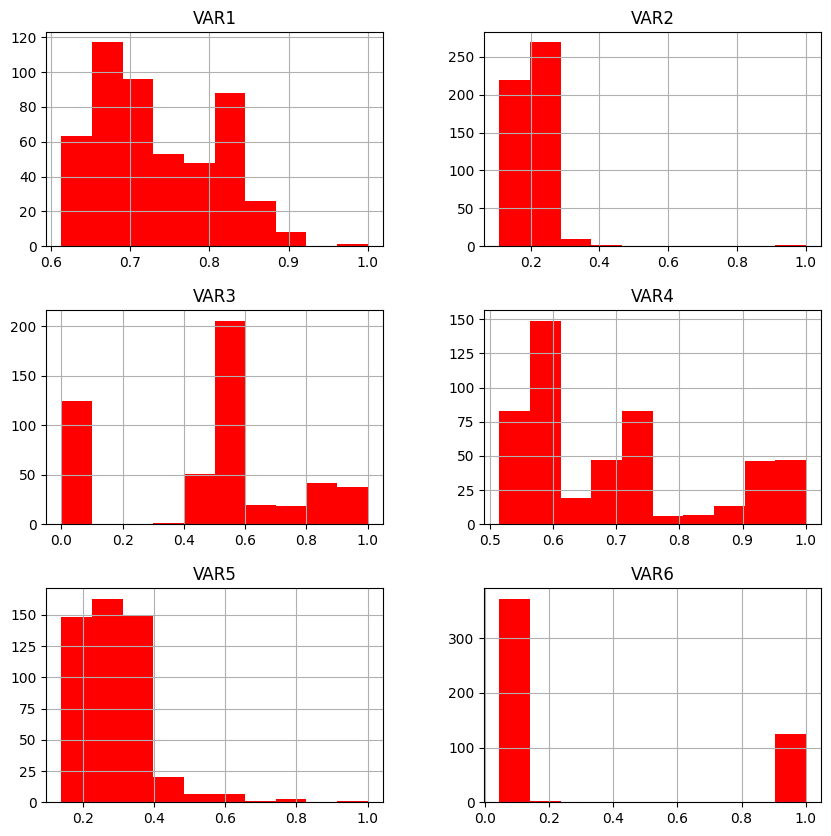
# Histograma de cada feature, para ver las distribuciones en cada feature y detectar alguna anómala o con pocos datos fuera de rango o incluso features nulas
import matplotlib.pyplot as plt
df2.hist(figsize = (10,10), color='red')
plt.show()

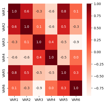
import seaborn as sns
# Matriz de correlación
df3=df2.drop(['CLASS'], axis=1)
#df3['VAR7']=2*df2['VAR1']
corr = df3.corr()

# Mapas de calor de la matriz de correlación
plt.figure(figsize=(5,5))
sns.heatmap(corr,fmt='.1f',annot=True,cmap='Reds')
plt.show()

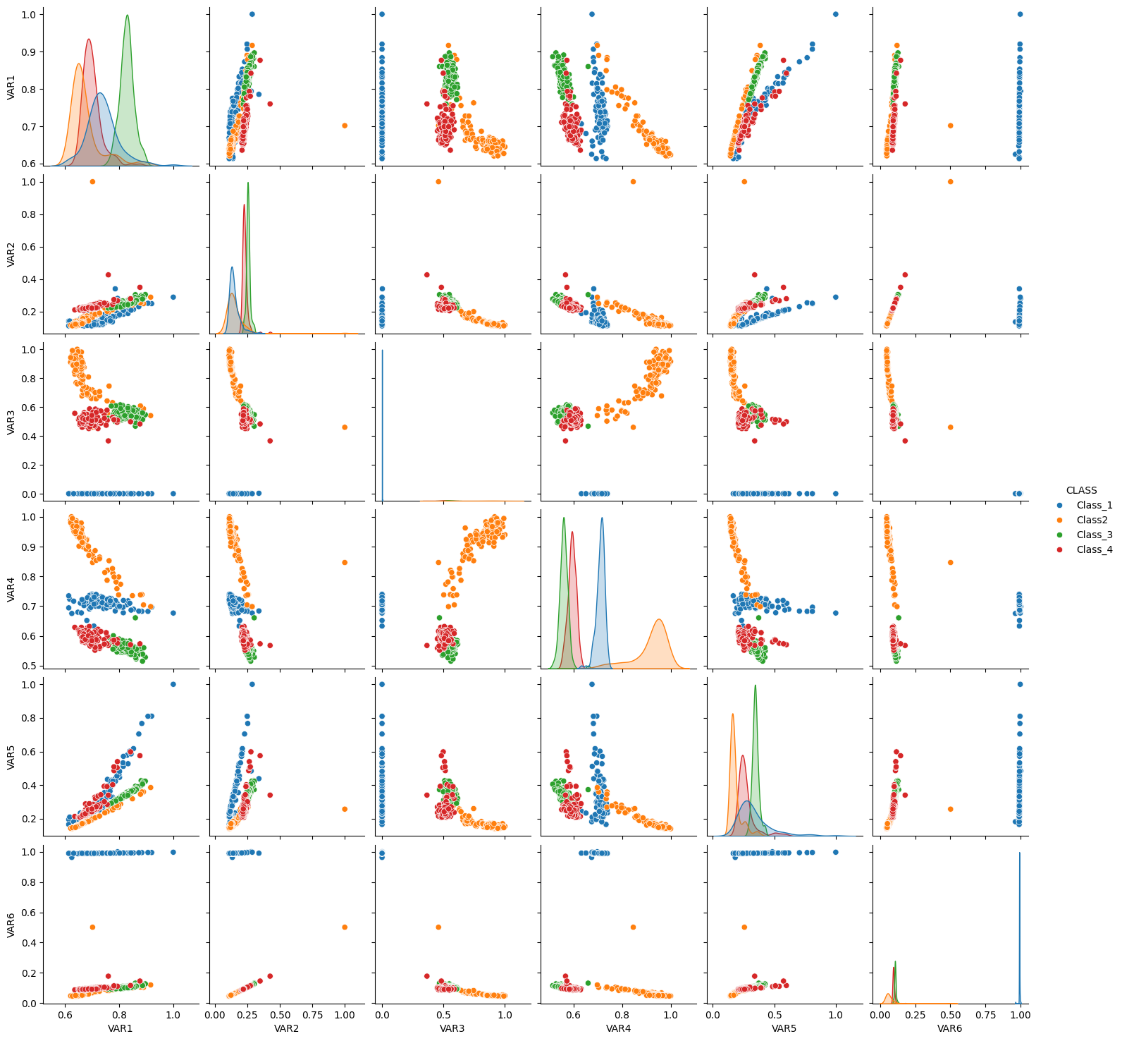
# Pairplot
sns.pairplot(df2, hue="CLASS")

<seaborn.axisgrid.PairGrid at 0x7a8d9bcffe80>

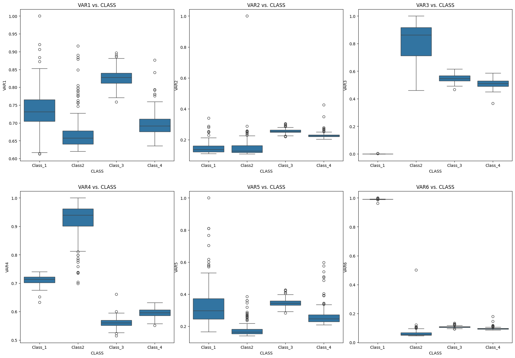
#plots
nrows=2
ncols=3

fig = plt.figure(figsize=(22,15))
fig.subplots_adjust(hspace=0.2, wspace=0.1)

###############################################
i=1
ax = fig.add_subplot(nrows, ncols, i)
sns.boxplot(data=df2, x="CLASS", y="VAR1")
ax.set_xlabel("CLASS")
ax.set_ylabel("VAR1")
ax.set_title('VAR1 vs. CLASS')
###############################################
i=2
ax = fig.add_subplot(nrows, ncols, i)
sns.boxplot(data=df2, x="CLASS", y="VAR2")
ax.set_xlabel("CLASS")
ax.set_ylabel("VAR2")
ax.set_title('VAR2 vs. CLASS')
###############################################
i=3
ax = fig.add_subplot(nrows, ncols, i)
sns.boxplot(data=df2, x="CLASS", y="VAR3")
ax.set_xlabel("CLASS")
ax.set_ylabel("VAR3")
ax.set_title('VAR3 vs. CLASS')
###############################################
i=4
ax = fig.add_subplot(nrows, ncols, i)
sns.boxplot(data=df2, x="CLASS", y="VAR4")
ax.set_xlabel("CLASS")
ax.set_ylabel("VAR4")
ax.set_title('VAR4 vs. CLASS')
###############################################
i=5
ax = fig.add_subplot(nrows, ncols, i)
sns.boxplot(data=df2, x="CLASS", y="VAR5")
ax.set_xlabel("CLASS")
ax.set_ylabel("VAR5")
ax.set_title('VAR5 vs. CLASS')
###############################################
i=6
ax = fig.add_subplot(nrows, ncols, i)
sns.boxplot(data=df2, x="CLASS", y="VAR6")
ax.set_xlabel("CLASS")
ax.set_ylabel("VAR6")
ax.set_title('VAR6 vs. CLASS')
plt.show()

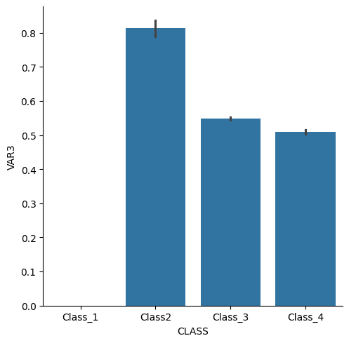
sns.catplot(data=df2, kind="bar", x="CLASS", y="VAR3")

<seaborn.axisgrid.FacetGrid at 0x7a8d93311210>

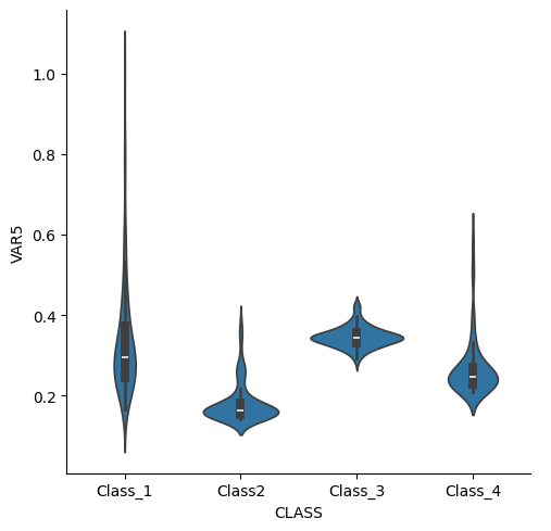
sns.catplot(data=df2, kind="violin", x="CLASS", y="VAR5")

<seaborn.axisgrid.FacetGrid at 0x7a8d90e36770>

División en datos de entrenamiento y testing

# Obtener las features
features = df.drop(['diagnosis'], axis=1)
features.head()

	radius_mean	texture_mean	perimeter_mean	area_mean	smoothness_mean	compactness_mean	concavity_mean	concave_points_mean	symmetry_mean	fractal_dimension_mean	radius_se	texture_se	perimeter_se	area_se	smoothness_se	compactness_se	concavity_se	concave_points_se	symmetry_se	fractal_dimension_se	radius_worst	texture_worst	perimeter_worst	area_worst	smoothness_worst	compactness_worst	concavity_worst	concave_points_worst	symmetry_worst	fractal_dimension_worst
0	17.99	10.38	122.80	1001.0	0.11840	0.27760	0.3001	0.14710	0.2419	0.07871	1.0950	0.9053	8.589	153.40	0.006399	0.04904	0.05373	0.01587	0.03003	0.006193	25.38	17.33	184.60	2019.0	0.1622	0.6656	0.7119	0.2654	0.4601	0.11890
1	20.57	17.77	132.90	1326.0	0.08474	0.07864	0.0869	0.07017	0.1812	0.05667	0.5435	0.7339	3.398	74.08	0.005225	0.01308	0.01860	0.01340	0.01389	0.003532	24.99	23.41	158.80	1956.0	0.1238	0.1866	0.2416	0.1860	0.2750	0.08902
2	19.69	21.25	130.00	1203.0	0.10960	0.15990	0.1974	0.12790	0.2069	0.05999	0.7456	0.7869	4.585	94.03	0.006150	0.04006	0.03832	0.02058	0.02250	0.004571	23.57	25.53	152.50	1709.0	0.1444	0.4245	0.4504	0.2430	0.3613	0.08758
3	11.42	20.38	77.58	386.1	0.14250	0.28390	0.2414	0.10520	0.2597	0.09744	0.4956	1.1560	3.445	27.23	0.009110	0.07458	0.05661	0.01867	0.05963	0.009208	14.91	26.50	98.87	567.7	0.2098	0.8663	0.6869	0.2575	0.6638	0.17300
4	20.29	14.34	135.10	1297.0	0.10030	0.13280	0.1980	0.10430	0.1809	0.05883	0.7572	0.7813	5.438	94.44	0.011490	0.02461	0.05688	0.01885	0.01756	0.005115	22.54	16.67	152.20	1575.0	0.1374	0.2050	0.4000	0.1625	0.2364	0.07678

# Obtener los labels
labels = df['diagnosis']
labels.head()

0    M
1    M
2    M
3    M
4    M
Name: diagnosis, dtype: object

features.shape,labels.shape

((569, 30), (569,))

from sklearn.model_selection import train_test_split
# Separación de la data, con un 20% para testing, y 80% para entrenamiento
X_train, X_test, y_train, y_test = train_test_split(features, labels,
                                                    test_size=0.20, random_state=1, stratify=labels)

X_train.shape, X_test.shape, y_train.shape, y_test.shape

((455, 30), (114, 30), (455,), (114,))

import numpy as np

# Verificacion de la cantidad de datos para entrenamiento y para testing
print("y_train labels unique:",np.unique(y_train, return_counts=True))
print("y_test labels unique: ",np.unique(y_test, return_counts=True))

y_train labels unique: (array(['B', 'M'], dtype=object), array([285, 170]))
y_test labels unique:  (array(['B', 'M'], dtype=object), array([72, 42]))

K-Nearest Neighbors

from sklearn.neighbors import KNeighborsClassifier
# Cargamos el modelo KNN sin entrenar
model_KNN = KNeighborsClassifier(n_neighbors=3)

# Entrenamos el modelo KNN
model_KNN.fit(X_train, y_train)

KNeighborsClassifier(n_neighbors=3)

In a Jupyter environment, please rerun this cell to show the HTML representation or trust the notebook.
On GitHub, the HTML representation is unable to render, please try loading this page with nbviewer.org.

# Hacemos predicción en testing
y_pred = model_KNN.predict(X_test)

# Mostramos las predicciones
y_pred

array(['M', 'B', 'B', 'M', 'B', 'M', 'M', 'M', 'B', 'B', 'B', 'B', 'M',
       'B', 'M', 'B', 'B', 'M', 'M', 'B', 'M', 'B', 'B', 'M', 'M', 'B',
       'B', 'B', 'B', 'B', 'B', 'B', 'B', 'B', 'B', 'B', 'M', 'B', 'B',
       'M', 'M', 'B', 'B', 'B', 'B', 'B', 'M', 'M', 'M', 'B', 'M', 'M',
       'M', 'B', 'B', 'B', 'B', 'M', 'B', 'M', 'B', 'M', 'M', 'B', 'B',
       'M', 'M', 'B', 'B', 'B', 'B', 'B', 'M', 'B', 'M', 'M', 'B', 'B',
       'M', 'B', 'B', 'B', 'M', 'B', 'B', 'M', 'B', 'B', 'M', 'M', 'B',
       'B', 'M', 'M', 'B', 'B', 'B', 'B', 'B', 'B', 'B', 'B', 'B', 'B',
       'B', 'B', 'M', 'M', 'B', 'B', 'B', 'B', 'B', 'M'], dtype=object)

y_test.to_numpy()

array(['M', 'B', 'B', 'M', 'B', 'M', 'M', 'M', 'B', 'B', 'B', 'B', 'M',
       'B', 'M', 'M', 'B', 'B', 'M', 'B', 'M', 'B', 'B', 'M', 'M', 'B',
       'B', 'B', 'B', 'B', 'B', 'B', 'B', 'B', 'B', 'B', 'M', 'B', 'B',
       'M', 'M', 'B', 'B', 'B', 'B', 'B', 'M', 'M', 'M', 'B', 'M', 'M',
       'M', 'B', 'B', 'B', 'M', 'M', 'B', 'B', 'B', 'M', 'M', 'B', 'B',
       'M', 'M', 'B', 'B', 'B', 'B', 'B', 'M', 'M', 'M', 'M', 'B', 'B',
       'M', 'B', 'B', 'B', 'B', 'B', 'B', 'M', 'B', 'B', 'M', 'M', 'M',
       'B', 'M', 'M', 'B', 'B', 'B', 'B', 'B', 'B', 'B', 'B', 'B', 'M',
       'B', 'B', 'M', 'M', 'B', 'B', 'B', 'B', 'B', 'M'], dtype=object)

# Hacemos predicción en testing para obtener las probabilidades
y_pred_proba = model_KNN.predict_proba(X_test)[:,1]

# Mostramos las predicciones
y_pred_proba.shape

(114,)

y_pred_proba

array([0.66666667, 0.        , 0.        , 1.        , 0.        ,
       1.        , 1.        , 1.        , 0.        , 0.        ,
       0.        , 0.        , 0.66666667, 0.        , 1.        ,
       0.        , 0.        , 0.66666667, 1.        , 0.        ,
       1.        , 0.        , 0.        , 0.66666667, 1.        ,
       0.        , 0.        , 0.        , 0.        , 0.        ,
       0.        , 0.        , 0.        , 0.        , 0.        ,
       0.        , 1.        , 0.        , 0.        , 1.        ,
       1.        , 0.33333333, 0.        , 0.        , 0.        ,
       0.        , 0.66666667, 1.        , 1.        , 0.        ,
       1.        , 1.        , 1.        , 0.        , 0.        ,
       0.        , 0.33333333, 1.        , 0.        , 0.66666667,
       0.        , 1.        , 1.        , 0.        , 0.        ,
       1.        , 0.66666667, 0.        , 0.        , 0.        ,
       0.        , 0.        , 1.        , 0.        , 1.        ,
       0.66666667, 0.        , 0.        , 0.66666667, 0.        ,
       0.        , 0.        , 1.        , 0.        , 0.        ,
       1.        , 0.        , 0.        , 1.        , 1.        ,
       0.        , 0.        , 1.        , 1.        , 0.        ,
       0.        , 0.33333333, 0.        , 0.        , 0.        ,
       0.        , 0.        , 0.        , 0.33333333, 0.        ,
       0.        , 1.        , 1.        , 0.        , 0.        ,
       0.        , 0.        , 0.33333333, 1.        ])

Métricas

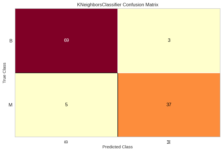
from sklearn.metrics import confusion_matrix
# Matriz de confusión
confusion_matrix(y_test,y_pred)

array([[69,  3],
       [ 5, 37]])

from sklearn.metrics import accuracy_score
# Accuracy
accuracy_s = accuracy_score(y_test,y_pred)
print('accuracy_score: {0:.4f}'.format(accuracy_s))

accuracy_score: 0.9298

Métricas bonitas

# Matriz de confusión
from yellowbrick.classifier import confusion_matrix as  cm
model = KNeighborsClassifier(n_neighbors=3)
visualizer_cm = cm(model, X_train, y_train, X_test, y_test)

from sklearn.preprocessing import LabelEncoder

le = LabelEncoder()
le.fit(list(np.unique(np.array(y_train)))) #['B', 'M']
y_train_coded = le.transform(y_train)
y_test_coded = le.transform(y_test)

# Reporte de clasificación
model = KNeighborsClassifier(n_neighbors=3)

from yellowbrick.classifier import classification_report as cr
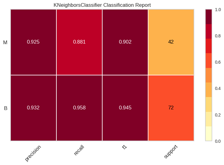
visualizer_cr = cr(model, X_train, y_train_coded, X_test, y_test_coded, classes=list(np.unique(np.array(y_train))), support=True)

# Error de predicción por clase
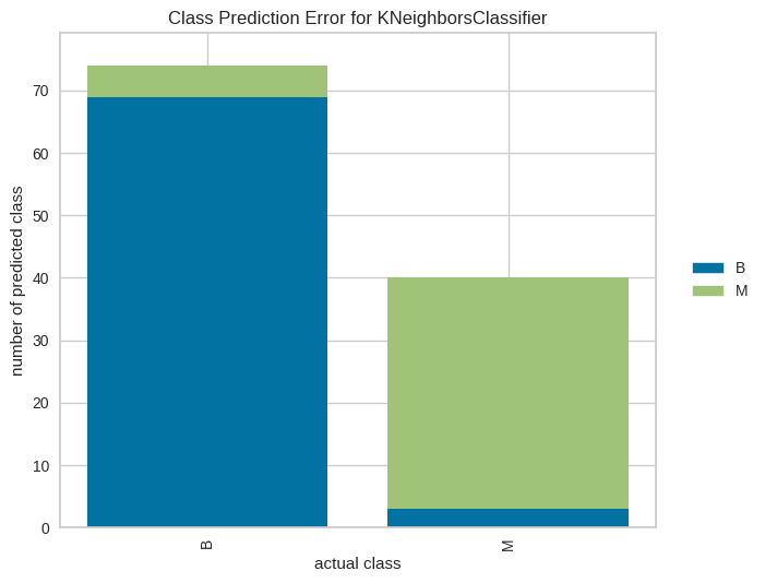
from yellowbrick.classifier import class_prediction_error
model = KNeighborsClassifier(n_neighbors=3)
visualizer_pe = class_prediction_error(model,X_train, y_train, X_test, y_test)

KNN con preprocesamiento de las caracteristicas

Data sin preprocesamiento de features

from sklearn import preprocessing
# Cargamos el modelo KNN sin entrenar
model_KNN = KNeighborsClassifier(n_neighbors=3)
# Entrenamos el modelo KNN
model_KNN.fit(X_train, y_train)
# Obtenemos la métrica lograda
print(model_KNN.score(X_test, y_test))
# Definir preprocesamiento
standard_scaler = preprocessing.StandardScaler()
# Preprocesar los datos
X_train_standard = standard_scaler.fit_transform(X_train)
X_test_standard = standard_scaler.transform(X_test)
# Cargamos el modelo KNN sin entrenar
model_KNN = KNeighborsClassifier(n_neighbors=3)
# Entrenamos el modelo KNN
model_KNN.fit(X_train_standard, y_train)
# Obtenemos la métrica lograda
print(model_KNN.score(X_test_standard, y_test))
# Definir preprocesamiento
min_max_scaler = preprocessing.MinMaxScaler()
# Preprocesar los datos
X_train_minmax = min_max_scaler.fit_transform(X_train)
X_test_minmax = min_max_scaler.transform(X_test)
# Cargamos el modelo KNN sin entrenar
model_KNN = KNeighborsClassifier(n_neighbors=3)
# Entrenamos el modelo KNN
model_KNN.fit(X_train_minmax, y_train)
# Obtenemos la métrica lograda
model_KNN.score(X_test_minmax, y_test)

0.9298245614035088
0.9649122807017544

0.9385964912280702

Balance de clases.

# Balance de clases hacia la clase mayor
from imblearn.over_sampling import RandomOverSampler

sampler = RandomOverSampler(random_state=1)
X_train_balanced, y_train_balanced = sampler.fit_resample(X_train, y_train)

print("y_test  original: ",np.unique(y_test, return_counts=True))
print("y_train original: ",np.unique(y_train, return_counts=True))
print("y_train balanced: ",np.unique(y_train_balanced, return_counts=True))

y_test  original:  (array(['B', 'M'], dtype=object), array([72, 42]))
y_train original:  (array(['B', 'M'], dtype=object), array([285, 170]))
y_train balanced:  (array(['B', 'M'], dtype=object), array([285, 285]))

# Balance de clases hacia la clase mayor
from imblearn.over_sampling import SMOTE

sampler = SMOTE(random_state=1)
X_train_balanced, y_train_balanced = sampler.fit_resample(X_train, y_train)

print("y_test  original: ",np.unique(y_test, return_counts=True))
print("y_train original: ",np.unique(y_train, return_counts=True))
print("y_train balanced: ",np.unique(y_train_balanced, return_counts=True))

y_test  original:  (array(['B', 'M'], dtype=object), array([72, 42]))
y_train original:  (array(['B', 'M'], dtype=object), array([285, 170]))
y_train balanced:  (array(['B', 'M'], dtype=object), array([285, 285]))

# Balance de clases hacia la clase mayor
from imblearn.over_sampling import ADASYN

sampler = ADASYN(random_state=1)
X_train_balanced, y_train_balanced = sampler.fit_resample(X_train, y_train)

print("y_test  original: ",np.unique(y_test, return_counts=True))
print("y_train original: ",np.unique(y_train, return_counts=True))
print("y_train balanced: ",np.unique(y_train_balanced, return_counts=True))

y_test  original:  (array(['B', 'M'], dtype=object), array([72, 42]))
y_train original:  (array(['B', 'M'], dtype=object), array([285, 170]))
y_train balanced:  (array(['B', 'M'], dtype=object), array([285, 293]))

# Balance de clases hacia la clase mayor
from imblearn.over_sampling import BorderlineSMOTE

sampler = BorderlineSMOTE(random_state=1)
X_train_balanced, y_train_balanced = sampler.fit_resample(X_train, y_train)

print("y_test  original: ",np.unique(y_test, return_counts=True))
print("y_train original: ",np.unique(y_train, return_counts=True))
print("y_train balanced: ",np.unique(y_train_balanced, return_counts=True))

y_test  original:  (array(['B', 'M'], dtype=object), array([72, 42]))
y_train original:  (array(['B', 'M'], dtype=object), array([285, 170]))
y_train balanced:  (array(['B', 'M'], dtype=object), array([285, 285]))

# Balance de clases hacia la clase mayor
from imblearn.over_sampling import KMeansSMOTE

sampler = KMeansSMOTE(random_state=1)
X_train_balanced, y_train_balanced = sampler.fit_resample(X_train, y_train)

print("y_test  original: ",np.unique(y_test, return_counts=True))
print("y_train original: ",np.unique(y_train, return_counts=True))
print("y_train balanced: ",np.unique(y_train_balanced, return_counts=True))

/usr/local/lib/python3.10/dist-packages/sklearn/cluster/_kmeans.py:870: FutureWarning: The default value of `n_init` will change from 3 to 'auto' in 1.4. Set the value of `n_init` explicitly to suppress the warning
  warnings.warn(

y_test  original:  (array(['B', 'M'], dtype=object), array([72, 42]))
y_train original:  (array(['B', 'M'], dtype=object), array([285, 170]))
y_train balanced:  (array(['B', 'M'], dtype=object), array([285, 290]))

# Balance de clases hacia la clase mayor
from imblearn.over_sampling import SVMSMOTE

sampler = SVMSMOTE(random_state=1)
X_train_balanced, y_train_balanced = sampler.fit_resample(X_train, y_train)

print("y_test  original: ",np.unique(y_test, return_counts=True))
print("y_train original: ",np.unique(y_train, return_counts=True))
print("y_train balanced: ",np.unique(y_train_balanced, return_counts=True))

y_test  original:  (array(['B', 'M'], dtype=object), array([72, 42]))
y_train original:  (array(['B', 'M'], dtype=object), array([285, 170]))
y_train balanced:  (array(['B', 'M'], dtype=object), array([285, 285]))

# Balance de clases hacia la clase mayor
from imblearn.over_sampling import SMOTEN

sampler = SMOTEN(random_state=1)
X_train_balanced, y_train_balanced = sampler.fit_resample(X_train, y_train)

print("y_test  original: ",np.unique(y_test, return_counts=True))
print("y_train original: ",np.unique(y_train, return_counts=True))
print("y_train balanced: ",np.unique(y_train_balanced, return_counts=True))

y_test  original:  (array(['B', 'M'], dtype=object), array([72, 42]))
y_train original:  (array(['B', 'M'], dtype=object), array([285, 170]))
y_train balanced:  (array(['B', 'M'], dtype=object), array([285, 285]))

# Balance de clases hacia la clase menor
from imblearn.under_sampling import RandomUnderSampler

sampler = RandomUnderSampler(random_state=1)
X_train_balanced, y_train_balanced = sampler.fit_resample(X_train, y_train)

print("y_test  original: ",np.unique(y_test, return_counts=True))
print("y_train original: ",np.unique(y_train, return_counts=True))
print("y_train balanced: ",np.unique(y_train_balanced, return_counts=True))

y_test  original:  (array(['B', 'M'], dtype=object), array([72, 42]))
y_train original:  (array(['B', 'M'], dtype=object), array([285, 170]))
y_train balanced:  (array(['B', 'M'], dtype=object), array([170, 170]))

# Balance de clases hacia la clase menor
from imblearn.under_sampling import ClusterCentroids

sampler = ClusterCentroids(random_state=1)
X_train_balanced, y_train_balanced = sampler.fit_resample(X_train, y_train)

print("y_test  original: ",np.unique(y_test, return_counts=True))
print("y_train original: ",np.unique(y_train, return_counts=True))
print("y_train balanced: ",np.unique(y_train_balanced, return_counts=True))

/usr/local/lib/python3.10/dist-packages/sklearn/cluster/_kmeans.py:870: FutureWarning: The default value of `n_init` will change from 10 to 'auto' in 1.4. Set the value of `n_init` explicitly to suppress the warning
  warnings.warn(

y_test  original:  (array(['B', 'M'], dtype=object), array([72, 42]))
y_train original:  (array(['B', 'M'], dtype=object), array([285, 170]))
y_train balanced:  (array(['B', 'M'], dtype=object), array([170, 170]))

# Balance de clases hacia la clase menor
from imblearn.under_sampling import NearMiss
sampler = NearMiss()
X_train_balanced, y_train_balanced = sampler.fit_resample(X_train, y_train)

print("y_test  original: ",np.unique(y_test, return_counts=True))
print("y_train original: ",np.unique(y_train, return_counts=True))
print("y_train balanced: ",np.unique(y_train_balanced, return_counts=True))

y_test  original:  (array(['B', 'M'], dtype=object), array([72, 42]))
y_train original:  (array(['B', 'M'], dtype=object), array([285, 170]))
y_train balanced:  (array(['B', 'M'], dtype=object), array([170, 170]))